SEMANTIC LABELLING OF ULTRA DENSE MLS POINT CLOUDS IN URBAN ROAD
CORRIDORS BASED ON FUSING CRF WITH SHAPE PRIORS
W.Yao a,b, P. Polewskia, P. Krzystek a
aMunich University of Applied sciences, 80333 Munich, Germany - (yao, polewski, krzystek)@hm.edu bDepartment of Land Surveying and Geo-Informatics, The Hong Kong Polytechnic University, Hung Hom, Hong Kong
KEY WORDS: Ultra denseMLS, urban road corridor, evidence fusion, object classification, probabilistic graph models
ABSTRACT:
In this paper, a labelling method for the semantic analysis of ultra-high point density MLS data (up to 4000 points/m2) in urban road corridors is developed based on combining a conditional random field (CRF) for the context-based classification of 3D point clouds with shape priors. The CRF uses a Random Forest (RF) for generating the unary potentials of nodes and a variant of the contrast-sensitive Potts model for the pair-wise potentials of node edges. The foundations of the classification are various geometric features derived by means of co-variance matrices and local accumulation map of spatial coordinates based on local neighbourhoods. Meanwhile, in order to cope with the ultra-high point density, a plane-based region growing method combined with a rule-based classifier is applied to first fix semantic labels for man-made objects. Once such kind of points that usually account for majority of entire data amount are pre-labeled; the CRF classifier can be solved by optimizing the discriminative probability for nodes within a subgraph structure excluded from pre-labeled nodes. The process can be viewed as an evidence fusion step inferring a degree of belief for point labelling from different sources. The MLS data used for this study were acquired by vehicle-borne Z+F phase-based laser scanner measurement, which permits the generation of a point cloud with an ultra-high sampling rate and accuracy. The test sites are parts of Munich City which is assumed to consist of seven object classes including impervious surfaces, tree, building roof/facade, low vegetation, vehicle and pole. The competitive classification performance can be explained by the diverse factors: e.g. the above ground height highlights the vertical dimension of houses, trees even cars, but also attributed to decision-level fusion of graph-based contextual classification approach with shape priors. The use of context-based classification methods mainly contributed to smoothing of labelling by removing outliers and the improvement in underrepresented object classes. In addition, the routine operation of a context-based classification for such high density MLS data becomes much more efficient being comparable to non-contextual classification schemes.
1. INTRODUCTION
Object semantic labeling is a very important issue for urban remote sensing. The results are appealing for a wide range of applications such as facility mapping, environment assessment and road inventory. While digital imaging sensors are frequently adopted to characterize the urban landscape and land use types, mobile laser scanners (MLS) are increasingly used to directly acquire dense 3D geo-data about urban facility along the road corridor (Babahajiani et al., 2016;Yu et al., 2015). MLS is generally used for small-scale area applications, such as road inventory in individual sections, and provide accurate and dense 3D data of the object surfaces. However, the point density is dependent on the distance of the scanner to the individual objects, resulting in an inhomogeneous 3D point cloud. The main application area for MLS is the inclusion of road peripheral environments, such as parts of urban or rural areas with focus on road facility but usually very high point densities.
Nowadays, due to the availability of large amounts of labeled data and powerful computers, the success of machine learning methods in classifying point clouds is already confirmed on diverse applications. The automatic interpretation of 3D point clouds is a highly current topic and is becoming increasingly important in the field of remote sensing, computer vision and robotics. Reasons for this include the development of MLS, the further increased adoption of Unmanned Aerial Systems for data acquisition. Several researchers have successfully applied the semantic annotation scheme to point cloud data. Early days started with predicting discrete class label for each point by using feature vector. Over recent years, with high resolution data there is an opportunity for fine-grained classification such as roads, building facades/roofs, trees, power lines, poles/tree stems and
cars using sophisticated features and machine learning algorithms(Wang et al., 2015; Yao et al., 2016). Especially in urban areas, there are many application areas that are based on 3D point clouds. These include, for example, the generation of 3D city models for the planning of infrastructure and urban development or the use of vehicle navigation. A basic step for most of the above applications is to perform a classification of the 3D point clouds in order to assign a semantic object class (e.g., car, building, vegetation or road) to each individual 3D point.
Former studies are frequently focused on individual object classes such as buildings, vegetation, or street lights/traffic signs (Steinsick et al., 2017; Yu et al., 2015). Weinmann et al. (2015) used Conditional Random Fields (CRF) for point-by-point classification of several objects in urban ALS or MLS data. The use of CRF shows a clear improvement in the classification results compared to conventional methods such as Random Forest (RF) and Support Vector Machines (SVM). However, the complex model of the CRF increases the calculation effort, which is becoming impossible for MLS data with such density. Moreover, for semantic labelling in point clouds, Lindenbergh et al. (2015) used super-voxel features of dense MLS data and classification-based segmentation scheme for tree detection and parameter extraction. However, up to 97% of point cloud data were reduced via voxelization which could lead to undersegmentation effect. Hackel et al. (2016) presented an efficient classification method for dense 3D points by constructing approximate multi-scale neighborhoods for extracting a rich feature representation in very little time. But in this work topological relations among the point clouds were unfortunately not considered.
The most common difficulties concerning the classification of MLS point clouds are mainly due to the large amount of data, variations in point density, incomplete structures due to occlusions, or due to differences between objects within the same class. Due to very complex structures and many different neighboring object classes, 3D scenes in urban areas are particularly challenging. The aim of this work is to develop a method for the dense semantic labeling of 3D point clouds in urban areas, which is applicable for ultra-high point density MLS data. The analysis includes all the necessary steps to assign an object class to each 3D point: (i) the selection of a suitable local point neighborhood for the (ii) extraction of distinctive features; and (iii) performing the context-based point -wise classification using an evidence fusion method.
The goal of this work is to develop a workflow for dense semantic labelling in city road corridors using very high fidelity MLS data, which is based on combining a shape-based categorization scheme with point-wise CRF classification using spatial-locality features. We propose an effective strategy to address time-consuming contextual classification task for urban scenes based on point labeling.
2. METHOD
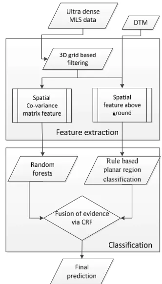
In this section, we present the framework for automated point classification in ultra-dense MLS point clouds. We first introduce locality-based spatial features with optimized neighborhood size. We then introduce the plane-based region growing operation adopted for shape prior extraction and fixing their labels using rule-based classifier. Finally, we use the concept of evidence fusion to refine initial labeling results by a constrained CRF method for subsets of graph nodes. An overview of the proposed semantic labeling framework is illustrated in Fig. 1.
The goal of the classification of point clouds is to assign each 3D point one object class label. In these procedures, each 3D point is classified independently of its neighborhood. Recently, however, mainly context-based classification methods were presented, in which the object classes of the points in the neighborhood are included in the assignment process of the labels. As a result, all points are classified simultaneously. In this work a context-aware classification scheme is applied based on combining a constrained CRF and RF classifier (Fig 1).
2.1 Local neighbourhood definition for feature extraction At the very beginning, we have to downsample a point cloud dataset by reduce the number of points by 5 times using a voxelized grid approach. The VoxelGrid operation that we used creates a 3D voxel grid (a voxel grid is a set of tiny 3D boxes in space) over the input point cloud data. Then, in each voxel, all the points present will be approximated with its center. This approach is a bit faster than approximating them with the centroid of the voxel, and it is supposed to sufficiently represent the underlying surface of object classes to be classified. The first step is to define a suitable local neighborhood for a point cloud with points = ( , , ) ∈ℝ3 with ∈ {1, ..., }. The definition of the neighborhood serves to describe the local 3D structure around a given point and thus forms the basis for the extraction of geometric features. In this work two neighborhood definitions are considered: Spherical neighborhoods with fixed radius and an optimal spherical neighborhood with varying radius, based on the k ∈ℕ nearest neighbors and Eigen-entropy (Weinmann et al., 2015).
Figure 1. Workflow for the proposed labelling framework.
The value for a point depends on the local 3D structure and the local point density. As a result, some proposed methods for automatically determining individual values for are based on the local geometric properties of point clouds. To derive these properties, the 3D covariance matrix C ∈ℝ3×3 is calculated for a given point and its nearest neighbors. The three eigenvalues λ1, λ2, λ3∈ℝ, with λ1≥λ2≥λ3≥0 represent the extent of a three-dimensional covariance ellipsoid along its main axes and are thus suitable for describing the local 3D structure. The Shannon entropy of the normalized eigenvalues 1, 2, 3 serves as a basis for the calculation of the Eigen-entropy λ,i.
,i 1ln( )1 2ln( )2 3ln( )3
E e e e e e e (1)
The Eigen-entropy is a measure of the disorder of the 3D points within the local neighborhood. The idea of this approach is to find the optimum value of k, which minimizes the disorder of the 3D points within the neighborhood. But the value is varied with an increment of Δ for each point in a set interval of to . The value corresponding to the minimum Shannon entropy is assumed to be the optimal value. Once the local point neighborhood has been defined for each point , features can be derived. In this work, the features described in Weinmann et al. (2015) have been used, which are a combination of 2D and 3D features. Based on the three eigenvalues of the 3D covariance matrix, a total of nine geometric features are determined: Linearity λ, planarity λ, and sphericity λ provide information on whether it is a linear 1D structure, a planar 2D structure, or a volumetric 3D structure. The other eigenvalue-based features are the omnivariance λ, anisotropy λ, eigenentropy λ, the sum of the eigenvalues Σλ and the change in the curvature λ. As a further feature, the verticality is defined as = 1- | |, which can be calculated using the third component of the normal vector. The International Archives of the Photogrammetry, Remote Sensing and Spatial Information Sciences, Volume XLII-2/W7, 2017
In the case of MLS data with small-scale extension, however, the absolute height is used. Furthermore, the standard deviation of the height σ and the maximum height difference Δ within the local neighborhood serve as features. Furthermore, 2D features are extracted from an accumulation map of 3D point clouds by dividing the projection plane into discrete square bins with a side length of s. For each point the following characteristics are derived from the bin assigned to it: the number of points N in the bin, the maximum height difference Δ and the standard deviation of the height σ ,Acc
2.2 Pre-classification using plane fitting and heuristic rules
The goal of this step is to extract planar structures from point clouds and assign semantic labels based on a set of heuristic rules. The motivation is twofold. First, planar surfaces make up a significant portion of the scene, while the semantic interpretation of vast horizontal or vertical planes as roads and facades is relatively straightforward. On the other hand, by removing large planes from the point cloud we are potentially simplifying the subsequent CRF based classification problem, because a decomposition of the entire scene into unconnected parts may be achieved. Each part may then be optimized independently.
For initial class probability calculation the application of random forest to the data is conducted in order to generate class-specific probabilities for each point. The plane extraction procedure is based on the region growing principle with a smoothness constraint due to Rabbani et al (2006). First, normal vector and curvature estimates are obtained for each point. Then, seed points are iteratively selected and their corresponding regions are expanded with neighboring points based on two criteria: maximum neighbor spatial distance d3d and maximum normal vector angular deviation dn compared to the seed point’s normal. Each recovered region with a point count above a predefined threshold is considered as a plane candidate and processed using a RANSAC plane fitting procedure. Finally, each plane is classified into one of 5 categories: car, roof, façade, ground or tree, based on the following simple rules. Let devz, havg, hmax, ptree denote, respectively: the plane normal’s angular deviation to the Z axis, the average and maximum above-ground height of the plane’s supporting points, as well as the average per-point probability of the ‘tree’ label obtained from random forest. Then, the heuristic rules can be defined as follows:
1. IF ptree > ptree,thr THEN class ← tree 2. ELSE IF | devz – 90°| < 10°
2a. IF hmax > 2 AND | devz – 90°| < 5° THEN class ← façade
2b. ELSE class ← car 3. ELSE
3a. IF havg < 0.15 THEN class ← ground 3b. ELSE IF havg > 3 THEN class ← roof 3c. ELSE class ← car
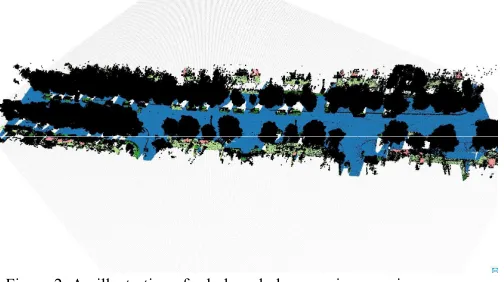
Figure 2. An illustration of rule-based planar region growing with all the non-planar points assigned to black
2.3 Constrained conditional random field with fixed labels
Spatial contextual features together with ensemble classifier were found as effective means in former study, for discriminating classes in semantical labeling for urban areas. Covariance matrix based features were extracted in a local neighborhood, which can be implemented using different classifiers such as random forests. Since those features used to generate unary probability could be complementary to the pair-wise interaction features modeled by the CRF, a separate graph-based optimization is done on the features to output class probabilities which are combined with those fixed labels imposed by shape priors.
CRFs are graph-based contextual classifiers which allow the modeling of dependencies between adjacent points. In contrast to standard classification, CRFs directly model the joint probability of the entire labeling Y of all objects simultaneously, conditioned on their features x (KUMAR & HEBERT 2006):
( | ) = ( ) ∏∈ ( , )∏∈ ∏∈ ( , , ) (2)
( ) corresponds to normalization constant referred to as a partition function. The equation consists of two functions: the association potential φ( , ) and the interaction potential ψ( , , ). The CRF is represented by an undirected graph = ( , ) with a set of nodes and a set of edges. The nodes i∈ correspond to the 3D points; the edges ij∈ connect two neighboring nodes and and model their dependencies. The point cloud has an irregular arrangement in three-dimensional space. In view of the high number of MLS points, the size of the local neighborhood within the graph is limited by a threshold for reasons of computing capacities. The vector contains the class labels for each 3D point, whereas x represents the independent variables. The aim of the classification is to find the optimal configuration Y, for which ( | ) becomes maximal.
Introducing fixed labels
Solving the optimization problem (2) for the set of all points may be computationally prohibitively expensive, especially for the case of high-density MLS point clouds. Therefore, it is desirable to decompose the problem into independent subproblems using the planar structures recovered in Sec. 2.2. For this purpose, consider a subset of labeled points PL of the entire point cloud, with index set L, i.e. = : ∈ . The labels of points from L correspond to the planar structure labels assigned in the previous step. Then, we can express the log-likelihood of labeling Y from (2) in the following manner:
ℓ( ) = ∑∉ ( ) +∑∈ ( ) + ∑∉ , ∉ , +
∑∉ , ∈ , +∑∈ , ∈ , + (3)
In the above, ( ) = ln
,
,
, = ln( , , )
and C is a constant. Since the labels of points from L are fixed, the terms in the energy function defined only over L are constant and do not influence the optimization. Moreover, the mixed pairwise term where each edge connects a fixed and a non-fixed node is transformed into a new unary potential ′:⋀∉ ( ) =
∑∈ , ~ ( , ), where ~ refers to the graph’s adjacency
relation. Therefore, a new optimization problem over a reduced set of labels ′ can be defined associated only with points having non-fixed labels.
Definition of potentials
The association potential φ( , ) connects the data and the corresponding class labels. For this potential, the result of any discriminative classifier can be used. The classifier must be able to provide a probability distribution over the possible values of the class label. A feature vector i( ) is created for each node based on the characteristics described in section 2.1. The association potential can be defined as the a posteriori probability of a local discriminative classifier based on i( ): φ( , ) = log( ( | ( ))).
A RF is used for the association potential φ ( , ). For RF, an ensemble of independent decision trees is created which are trained on random samples of the data, based on the bagging principle. The subsequent classification is done by means of a majority decision in which each tree votes for a class. The interaction potential ψ ( , , ) describes the local context by characterizing the interaction between the labels of two adjacent nodes , and features x. In this work a variant of the often used contrast-sensitive Potts model (BOYKOV & JOLLY 2001) is applied:
, , = ∙ ∙ + (1 − ) ∙
− ( )²² (4)
Here, δ corresponds to the Kronecker delta, which has the value one if = and otherwise assumes zero. j( ) is the Euclidean distance between the two feature vectors ( ) of the node and ( ) of the node connected by a common edge. The value is the average number of edges to which a node is connected in the graph, and the number of nodes in the local neighborhood of node i. The parameter σ is the average distance between the feature vectors of adjacent points. The two parameters 1 and 2 are weight parameters. The first weight determines the influence of the interaction potential on the classification and can assume any nonnegative, real value. The second weight 2∈[0; 1] influences the degree of smoothing depending on the data.
Training and inference
Firstly, the corresponding parameters and weights of the different classifiers must be determined in a training process. For the RF, the decision trees must be learned. A training set is generated with randomly selected 3D points per class. By balancing the classes, decision trees that are trained with very few or no examples of an underrepresented class are avoided. For the determination of the two weights 1 and 2 a method such as cross-validation can be used. For the classification by means of
CRF, the optimal assignment of the labels is determined which maximizes criterion (5). For graphs with cycles, the exact inference cannot be solved in a practical time, which is why generally only approximate solutions are used. In this work the Quadratic Pseudo-Boolean Optimization (BOROS & HAMMER 2002) is applied.
The point-based RF classifiers and shape priors provide us with evidences for semantical class labels from two different sources. The idea of the class labelling technique in this work is to apply the fusion of two independent outcomes of inference schemes, which amounts to combining local shape priors with spatial co-variance features to further boost the CRF classification accuracy and efficiency.
3. EXPERIMENTS 3.1 Dataset
In this study, the proposed method was applied to the MLS dataset, which were acquired by vehicle-borne Z+F phase-based laser scanner measurement, permitting the generation of a point cloud of urban road environment with an ultra-high sampling rate and accuracy. The MLS data contains several object classes: roof (4.6%), pole/mast/tree stem (10%), façade (8.4%), ground (50.5%), vehicle (1.2%), tree (20%) and low vegetation (5.3%). The data set was recorded in the vicinity of the downtown area of Munich city. The data are divided into a training data record with approximately 2.5M points, a validation data set with 25M points and test data sets with a total of approximately 28M points covering a road length of nearly 250m. Labelled ground truth data were not provided for the areas, but is supposed to be made up of 7 categories above. Therefore, the evaluation of results can only be made via visual analysis and comparison. DTM was calculated as well, where the normalized height of points is computed.
3.2 Experimental design and parameter setting
For the experimental design, we split the point cloud into training and validation sets, which are not completely intersected with each other. Since we do not have ground truth data, the evaluation is based on the visual inspection. The training test data were equally subdivided into subsets by re-balancing, each of which represents a semantic class to be classified.
The experiments are carried out with the two local neighborhoods. For the optimal neighborhood , the interval for is defined by = 10 and =100 with a step size of Δ = 1. For the spherical neighborhood Ns, the radius for the MLS data set = (0.4m; 0.6m; 0.8m) are investigated. The feature extraction is based on the nearest neighbors, which result from the corresponding neighborhood definition. The lateral s of the square bins for the features , Δ and σ , was determined empirically and set to = 0.25.
For all experiments, a constant training quantity with = 2000 randomly selected examples per class is generated for the RF. With an increase in the value, no significantly better classification results could be achieved. The number of decision trees was determined empirically and set to =100. The two weight parameters 1 and 2 of the Potts model are determined by means of a grid search on the entire training data record. For this purpose, the two parameters are varied with a certain interval each and the CRF is trained with all the resulting combinations. On the basis of the training accuracies, the best combination is then selected. For MLS data set 1=0.85 and 2= 0.1. The The International Archives of the Photogrammetry, Remote Sensing and Spatial Information Sciences, Volume XLII-2/W7, 2017
threshold for the maximum neighborhood size within the graph is set to ℎ = 25. Empirical thresholds ptree,thr for rule-based planar region growing for pre-fixed labels is set to 0.7.
3.3 Results
The constrained CRF is applied to combining RF inference probabilities, shape priors and pairwise interaction probabilities. The quantitative validation accuracy obtained using the base line of parameter settings is given in section 3.2. It seems that the aesthetic appeal of the labelling is explicitly improved by the fusion, although it is still lack of the numeric evidences arguably making it worthwhile. The main improvements brought by evidence fusion are to alleviate the regions labelling with ambiguous or conflicting probabilities, by removing mislabelled and fragmented regions
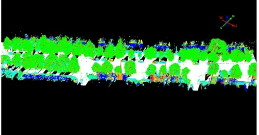
The result of the point-wise RF classifier solely using spatial-locality features on one test dataset is shown in Fig.3. The performance is qualitatively not bad considering the relative simplicity of the features and fixed local neighbourhood size. Fig.4 also shows a result after the decision fusion method is used to label the points. However, shape features show much higher representativeness of information content towards different object classes.
Figure 3. An illustration of result of RF classification
Figure 4. An illustration of result of fusion via constrained CRF
However, the training time increased rapidly as well when a bigger test site was applied to train the model. All computations were performed using an eight core CPU of an Intel Xeon E3-1245 with 3.40GHz. The validation of the training model on a test plot consisting of ca. 25 million MLS points takes one and half hour.
3.4 Discussion
The difference between the two classification methods in the overall performance is less than moderate. However, the differences in the individual classes are more. In particular, the underrepresented classes low vegetation and car show decent increases, respectively. In both procedures it is striking that especially the classes - low vegetation including shrub and Fence/hedge can be separated badly. In Fig. 3 and 4 the two classification results can be compared. The influence of the context-based classification is particularly visible in the classes: trees (green), façade (blue), and roof (yellow).
The good overall performance are strongly influenced by the very well-classified object class ground surface, which accounts for half of the entire points in the test data set. In both methods, the classes of low vegetation and poles/stems are less well recognized with only a small number of points. In comparison with RF, higher accuracy can be achieved with the aid of the CRF, especially for such classes. Overall, the CRF classification results look smoother for the MLS data than for RF. This smoothing effect is especially visible in the facades (blue) and tree (green) classes.
For the MLS dataset, the results of Munoz et al. (2009) showed that the context-based classification of point clouds is carried out using Functional Max-Margin Markov Networks. The results showed only major differences between the classes of high voltage line and pole/mast. While with the CRF used in this work, the class pole/ mast must have a much higher score, as the power line is not existent. Ramiya et al. (2016) used a 3D segmentation for the classification of the data set and extract spectral and geometric features from the segments. In addition to the 3D point cloud, a true orthophoto was used. For classification, multiclass machine learning method is applied with a one-vs-one strategy, combined with a genetic algorithm for feature selection. Radiometric, structural and geometric attributes are used as features. Other than the results of this work, the underrepresented classes of pole/mast, car and fence/hedge, measured on the basis of visual inspection, are less well detected, whereas the classes - low vegetation and roof are better recognized.
Meanwhile, in contrast to the traditional CRF approach which is usually very computationally time-consuming, constrained CRF model with prefixed labels achieved good accuracy but with significantly low computational costs. This is not surprising on one side, because the input features are explicitly designed to discriminate the target classes: the local distribution of normal vectors from point clouds highlights low vegetation and trees, above ground height highlights the building roof and cars and on the other side shape priors identify most of man-made objects such as façade, roof and road surface by fixing the class labels for CRF in advance.
Constrained CRF worked as a global smoothing filter to combine the two independent sources to generate final labels. The performed experiments give the rise to the fact that point labelling based on CRFs can even generate promising labelling results for all classes without inducing extra high time complexity.
4. CONCLUSION
The method proposed in this work provides good results for the ultra-dense MLS data. The adjustments with regard to the two different methods are only limited to the optimization of the two weight parameters. By incorporating context information, the The International Archives of the Photogrammetry, Remote Sensing and Spatial Information Sciences, Volume XLII-2/W7, 2017
classification result can be improved in all aspects with regard to individual classification. Particularly underrepresented classes with a few points in the data set benefit mostly from the context-based classification. The constrained CRF method provides a framework for combining the point-wise class labelling results of RF and local contexts. The improved classification performance is explained by the nature of input data: e.g. the vertical height and local variation of normal vectors, and as well as attributed to decision-level fusion of context-based classification approach with shape priors, which can not only generate more coherent labelling probability, but also confine the labeling to local constraints. A further development of the presented method could address the transferability of the trained classifier to different areas and sensors.
ACKNOWLEDGEMENTS
We would like to thank Dr. Gunnar Graefe from 3D Mapping Solutions GmbH for their productive contributions and providing us the MLS data.
REFERENCES
Babahajiani, P., Fan, L., Kamarainen, J. K. & Gabbouj, M., 2016. Comprehensive Automated 3D Urban Environment Modelling Using Terrestrial Laser Scanning Point Cloud. In Proceedings of the IEEE Conference on Computer Vision and Pattern Recognition Workshops, 10-18.
Lindenbergh, R. C., Berthold, D., Sirmacek, B., Herrero-Huerta, M., Wang, J. & Ebersbach, D., 2015. Automated large scale parameter extraction of road-side trees sampled by a laser mobile mapping system. The International Archives of Photogrammetry, Remote Sensing and Spatial Information Sciences, 40(3), 589. Boros, E. & Hammer, P. L., 2002. Pseudo-boolean optimization. Discrete Applied Mathematics 123(1-3), 155-225.
Boykov, Y. Y., & Jolly, M. P., (2001). Interactive graph cuts for optimal boundary & region segmentation of objects in ND images. In Computer Vision, ICCV 2001. Proceedings. Eighth IEEE International Conference on, vol. 1, pp. 105-112. Hackel, T., Wegner, J D. & Schindler, K., 2016. Fast semantic segmentation of 3D point clouds with strongly varying density. ISPRS Annals of the Photogrammetry, Remote Sensing and Spatial Information Sciences, Prague, Czech Republic, 2016, 3,177-184.
Kumar, S. & Hebert, M., 2006. Discriminative Random Fields. International Journal of Computer Vision 68(2), 179-201. Munoz, D., Bagnell, J. A., Vandapel, N. & Hebert, M., 2009. Contextual Classification with Functional Max-Margin Markov Networks. IEEE Conference on Computer Vision and Pattern Recognition 2009, 975-982.
Rabbani, T., Van Den Heuvel, F., & Vosselmann, G. 2006. Segmentation of point clouds using smoothness constraint. International archives of photogrammetry, remote sensing and spatial information sciences, 36(5), 248-253.
Ramiya, A. M.; Nidamanuri, R. R. & Krishnan, R., 2016. 3D semantic labelling of colored LiDAR point cloud using supervoxels based segmentation approach/color based region growing segmentation approach. http://ftp.ipi.uni-hannover.de/ISPRS_WGIII_website/ISPRSIII_4_Test_results/p apers/IIST_3D_ext.pdf (letzter Zugriff 20.01.2017)
Steinsiek, M.; Polewski, P.; Yao, W & Krzystek, P., 2017. Semantische Analyse von ALS- und MLS-Daten in urbanen Gebieten mittels Conditional Random Fields. 37. Wissenschaftlich-Technische Jahrestagung der DGPF in Würzburg – Publikationen der DGPF, Band 26, 2017 521. Wang, Z., Zhang, L., Fang, T., Mathiopoulos, P. T., Tong, X., Qu, H., & Chen, D., 2015. A multiscale and hierarchical feature extraction method for terrestrial laser scanning point cloud classification. IEEE Transactions on Geoscience and Remote Sensing, 53(5), 2409-2425.
Weinmann, M., Schmidt, A. & Mallet, C., 2015. Contextual classification of point cloud data by exploiting individual 3D neighborhoods. ISPRS Annals of Photogrammetry, Remote Sensing and Spatial Information Sciences II-3/W4, 271-278. Yao, W., Polewski, P. & Krzystek, P., 2016. Classification of Urban Aerial Data Based on Pixel Labelling with Deep Convolutional Neural Networks and Logistic Regression. ISPRS-International Archives of the Photogrammetry, Remote Sensing and Spatial Information Sciences, 405-410.
Yu, Y., Li, J., Guan, H & Wang, C., 2015. Automated Extraction of Urban Road Facilities Using Mobile Laser Scanning Data, IEEE Transactions on Intelligent Transportation Systems, 16(4), 2167-2181.