REGIONAL ECONOMIC MODELLING FOR INDONESIA: IMPLEMENTATION OF IRSA-INDONESIA5 | Resosudarmo | Journal of Indonesian Economy and Business 6259 67630 1 PB

(1)

Volume 26, Number 3, 2011, 287 – 309

REGIONAL ECONOMIC MODELLING FOR INDONESIA:

IMPLEMENTATION OF IRSA-INDONESIA5

*

Budy P. Resosudarmo The Australian National University

Canberra, Australia (budy.resosudarmo@anu.edu.au

)

Arief A. Yusuf Padjadjaran University Bandung, Jawa Barat, Indonesia

(arief.yusuf@fe.unpad.ac.id)

Djoni Hartono University of Indonesia Depok, Jawa Barat, Indonesia

(djoni.hartono@gmail.com)

Ditya A. Nurdianto The Australian National University

Canberra, Australia (ditya.nurdianto@kemlu.go.id)

ABSTRACT

Ten years after Indonesia implemented a major decentralisation policy, regional income per capita disparity and excessive rate of natural resource extraction continue to be pressing issues. There are great interests in identifying macro policies that would reduce regional income disparity and better control the rate of natural extraction, while maintaining reasonable national economic growth. This paper utilises an inter-regional computable general equilibrium model, IRSA-INDONESIA5, to discuss the economy-wide impacts of various policies dealing with the development gap among regions in the country, achieving low carbon growth, and reducing deforestation. The results of simulations conducted reveal that, primarily, the best way to reduce the development gap among regions is by creating effective programs to accelerate the growth of human capital in the less developed regions. Secondly, in the short-term, the elimination of energy subsidies and/or implementation of a carbon tax is effective in reducing CO2 emission and

producing higher economic growth, while in the long-run, however, technological improvement, particularly toward a more energy efficient technology, is needed to maintain a relatively low level of emission with continued high growth. Thirdly, if reducing deforestation means reducing the amount of timber harvested, it negatively affects the economy. To eliminate this negative impact, deforestation compensation is needed.

Keywords: computable general equilibrium, development planning and policy, environmental economics

*_{Budy P. Resosudarmo, Arief A. Yusuf and Djoni Hartono built the inter-regional computable general equilibrium}

(2)

INTRODUCTION

Indonesia is the world’s largest archi-pelagic state and one of the most spatially di-verse nations on earth in its resource endow-ments, population settleendow-ments, location of economic activity, ecology, and ethnicity. The disparity in socio-economic development sta-tus and environmental conditions has long been a crucial issue in this country (Hill et al.

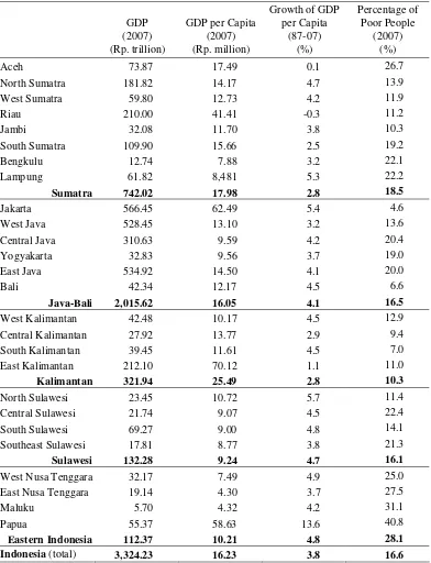
2008; Resosudarmo and Vidyattama, 2006; Resosudarmo and Vidyattama, 2007). In 2007, the gross domestic product (GDP) of the two richest provinces outside Java—Riau and East Kalimantan—was more than 36 times that of the poorest province, Maluku. Based on GDP per capita, East Kalimantan outstripped the rest of the country by far, Java included. East Kalimantan was almost twice as rich as the runner-up, Riau, and more than 16 times richer than Maluku in terms of per capita regional GDP. Some regions in the country are richly endowed with natural resources, such as oil, gas, coal and forests, while others are not. The range of poverty incidence also varies widely, from 4.6 percent of the population in Jakarta to 40.8 percent in Papua. Table 1 shows the economic indicators of several Indonesian regions.

It is well known that Indonesia has abun-dant natural resources such as oil, gas and minerals as well as rich and very diverse for-estry and marine resources. These resources, however, are not equally distributed across regions in the country. Oil and gas are found in Aceh, Riau, South Sumatra and East Kali-mantan. Mineral ores such as copper and gold are abundant in Papua, coal in most of Kali-mantan and West Sumatra, tin on the island of Bangka, nickel in South Sulawesi and North Maluku. Forests are mostly located in Sutra, Sulawesi, Kalimantan and Papua, and ma-rine resources in Eastern Indonesia. The two major criticisms with regard to natural re-source extraction in Indonesia are the skewed distribution of benefits and the

unsustainabil-ity of the rate of extraction (Resosudarmo, 2005).

Due to the demands of disadvantaged regions for larger income transfers and greater authority in constructing their development plans, and from rich natural resource regions to control their own natural endowments, rapid political change took place a few years after the economic crisis of 1997: Indonesia drasti-cally shifted from a highly centralistic govern-ment system to a highly decentralised one in 2001. Greater authority was delegated to more than 400 districts and municipalities, in the areas of education, agriculture, industry, trade and investment as well as infrastructure (Alm

et al. 2001). Only security, foreign relations, monetary and fiscal policies remain the responsibility of the central government (PP No. 25/2000).

Suddenly leaders of district and city levels of government acquired vast authority and responsibility, including receiving a huge transfer of civil servants from sectoral depart-ments within their jurisdiction. Provincial governments, however, generally remained relatively weak. In the new structure, regional governments received a much larger propor-tion of taxes and revenue sharing from natural extraction activities in their regions, with it being typical for budgets to triple after decen-tralisation. Yet the issues of regional income per capita disparity and the excessive rate of natural resource extraction remain (Resosudarmo and Jotzo, 2009).

(3)

Table 1. Indonesia’s Regional Outlook

GDP GDP per Capita

Growth of GDP per Capita

Percentage of Poor People

(2007) (2007) (87-07) (2007) (Rp. trillion) (Rp. million) (%) (%)

Aceh 73.87 17.49 0.1 26.7 North Sumatra 181.82 14.17 4.7 13.9 West Sumatra 59.80 12.73 4.2 11.9 Riau 210.00 41.41 -0.3 11.2 Jambi 32.08 11.70 3.8 10.3 South Sumatra 109.90 15.66 2.5 19.2 Bengkulu 12.74 7.88 3.2 22.1 Lampung 61.82 8,481 5.3 22.2 Sumatra 742.02 17.98 2.8 18.5 Jakarta 566.45 62.49 5.4 4.6 West Java 528.45 13.10 3.2 13.6 Central Java 310.63 9.59 4.2 20.4 Yogyakarta 32.83 9.56 3.7 19.0 East Java 534.92 14.50 4.1 20.0 Bali 42.34 12.17 4.5 6.6 Java-Bali 2,015.62 16.05 4.1 16.5 West Kalimantan 42.48 10.17 4.5 12.9 Central Kalimantan 27.92 13.77 2.9 9.4 South Kalimantan 39.45 11.61 4.5 7.0 East Kalimantan 212.10 70.12 1.1 11.0 Kalimantan 321.94 25.49 2.8 10.3 North Sulawesi 23.45 10.72 5.7 11.4 Central Sulawesi 21.74 9.07 4.5 22.4 South Sulawesi 69.27 9.00 4.8 14.1 Southeast Sulawesi 17.81 8.77 3.8 21.3 Sulawesi 132.28 9.24 4.7 16.1 West Nusa Tenggara 32.17 7.49 4.9 25.0 East Nusa Tenggara 19.14 4.30 3.7 27.5 Maluku 5.70 4.32 4.2 31.1 Papua 55.37 58.63 13.6 40.8 Eastern Indonesia 112.37 10.21 4.8 28.1 Indonesia (total) 3,324.23 16.23 3.8 16.6

(4)

suggest that an inter-regional computable gen-eral equilibrium model, in particular IRSA-INDONESIA5 which was developed under the Analysing Path of Sustainable Indonesia (APSI) project, is one of the most appropriate tools to analyse these issues. This paper aims to explain IRSA-INDONESIA5 and to discuss the economy-wide impacts of various policies dealing with the development gap among re-gions in the country, achieving low carbon growth, and reducing deforestation.

THE COMPUTABLE GENERAL EQUILIBRIUM MODEL

Market equilibrium represents a market condition such that the quantity of goods de-manded equals the quantity supplied at a price at which suppliers are prepared to sell and consumers to buy. Thus, it is the current state of exchange between buyers and sellers per-sists. When all markets in an economy are in equilibrium, this is known as a condition of general equilibrium. A computable general equilibrium (CGE) model uses realistic eco-nomic data to model the necessary criteria for an economy to attain a condition of general equilibrium. The CGE consists of a system of mathematical equations representing all agents’ behaviour; i.e. consumers’ and produc-ers’ behaviours and the market clearing condi-tions of goods and services in the economy. This system of equations is usually divided into five blocks of equations, namely:

 The Production Block: Equations in this block represent the structure of production activities and producers’ behaviour.

 The Consumption Block: This block con-sists of equations that represent the behav-iour of households and other institutions.

 The Export-Import Block: This block models the country’s decision to export or import goods and services.

 The Investment Block: Equations in this block simulate the decision to invest in the

economy, and the demand for goods and services used in the construction of the new capital.

 The Market Clearing Block: Equations in this block determine the market clearing conditions for labour, goods, and services in the economy. The national balance of pay-ments also falls within this block.

An inter-regional CGE model is one that models multi-region economies within a country. In this model, regions which consist of multiple sectors are typically inter-con-nected through trade, movements of people and capital, and government fiscal transfers. In general there are two approaches to construct-ing an inter-regional CGE model: the down and the bottom-up approaches. The top-down model solves the general equilibrium condition at the national level, which means the optimisation is done at this level. National results for quantity variables are broken down into regions using a share parameter. This ap-proach, therefore, recognises regional varia-tions in quantity but not in price.

(5)

1. CGE on Indonesia

The CGE model of the Indonesian economy became available at the end of the 1980s. Included among the first generation of Indonesian CGEs are those developed by BPS, ISS and CWFS (1986), Behrman, Lewis and Lotfi (1988)1, Ezaki (1989), and Thorbecke (1991). They were developed in close collabo-ration with the Indonesian National Planning and Development Agency (Bappenas), the Ministry of Finance and the Central Statistics Agency (BPS or Badan Pusat Statistik). They were all static CGE models. The models of Behrman et al. (1988) and Ezaki (1989) were based on the Indonesian input-output (IO) ta-bles, meaning their classifications of labour and household were limited and their models of household consumption were not complete. The models by BPS, ISS and CWFS (1986) and Thorbecke (1991) were based on the In-donesian social accounting matrix (SAM) which is generally a more complete system of data than an input-output table. The models by Behrman et al. (1988) and Thorbecke (1991) were written using GAMS software, while BPS, ISS and CWFS (1986) and Ezaki (1989) used other computer languages. The models of Ezaki (1989) and Thorbecke (1991), in addi-tion to the real sector, also include the finan-cial sector in order to determine absolute prices endogenously. All of these CGE models were developed to analyse the structural ad-justment program implemented by Indonesia as a response to the decline in the oil price in the early 1980s.

The second generation models of Indone-sian CGEs came out in the 2000s. Among oth-ers are the following: Abimanyu (2000) in collaboration with the Centre of Policy Studies (CPS) at Monash University developed an INDORANI CGE model based on the Indone-sian IO table. It is an application of the Aus-tralian ORANI model for Indonesia (Dixon et

1_{See Lewis (1991) for detail specification of the CGE}

utilized.

al. 1982), and so works on the platform of GEMPACK Software. There are two other derivatives of the ORANI model for Indone-sia, which are the Wayang model by Warr (2005) and the Indonesia-E3 by Yusuf (Yusuf and Resosudarmo, 2008). The advantage of Wayang over INDORANI is that Wayang is based on the Indonesian social accounting matrix and so has more household classifica-tions. The Indonesia-E3 disaggregated the Indonesian SAM households even further into 100 urban and 100 rural households so as to produce gini and poverty indexes. All of these CGE models are static in nature. INDORANI includes pollution emission equations for NO2, CO, SO2, SPM and BOD, and Indonesia-E3 for CO2 emissions.

In the GAMS software environment, Azis (2000) combined the models by Lewis (1991) and Thorbecke (1991) to develop a new dy-namic financial CGE model for Indonesia and analysed the impact of the 1997–98 Asian financial crisis on the Indonesian economy. The advantage of this CGE is the inclusion of the financial sector, so it can simulate financial policies. The Indonesian Central Bank cur-rently utilises this model for their policy analysis. Another dynamic CGE model for Indonesia was developed by Resosudarmo (2002 and 2008). It omits the financial sector, but does include close-loop relationships between the economy and air pollutants such as NO2, SO2 and SPM (2002) and between the economy and pesticide use (2008).

(6)

CPS at Monash University. It is a provincial level CGE, static in nature, a derivative of the inter-regional version of the ORANI model, based on the Indonesia IO table, and utilises GEMPACK Software. The models by Wuryanto and Pambudi are both bottom-up IRCGE models.

Note that other CGE models for Indonesia of equal importance to the ones mentioned above are available. They have not been men-tioned simply because the authors of this paper are not that familiar with them.

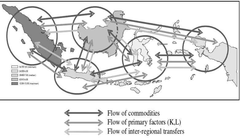
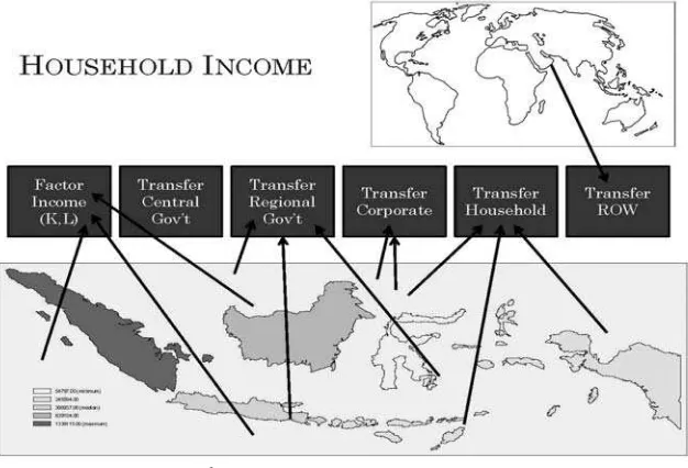
2. IRSA-INDONESIA5: Main Features IRSA-INDONESIA5 is a multi-year (dy-namic) CGE dividing Indonesia into five re-gions: Sumatra, Java-Bali, Kalimantan, Su-lawesi and Eastern Indonesia. Figure 1 illus-trates these divisions. The connections between regions are due to the flow of goods and services (or commodities), flow of capital and labour (or factors of production) and flows

of inter-regional transfers which can be among households, among governments, or between governments and households. It is important to note that each region is also connected with the rest of the world; i.e. they conduct import and export activities with other countries as well as sending money to and receiving it from friends and relatives abroad.

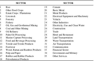
In each region there are 35 sectors of pro-duction, 16 labour classifications, accounts for capital and land, two types of households (ru-ral and urban households) and accounts for regional government and corporate enterprise. The 35 sectors, as seen in Table 2, are based on an inter-provincial input-output table de-veloped by the Indonesian statistical agency (BPS) for the national planning and develop-ment agency (Bappenas). There are four types of labour—agricultural, manual, clerical and professional workers—who are part of formal and informal sectors and are located in rural and urban areas.

54797.00 (minimum) 245594.00 398937.00 (median) 639154.00 1339115.00 (maximum)

Flow of commodities

Flow of primary factors (K,L)

Flow of inter-regional transfers

Source: Resosudarmo et al. (2009)

(7)

Table 2. Sectors in the Indonesian Inter-Regional CGE

SECTOR SECTOR

1 Rice 19 Cement 2 Other Food Crops 20 Basic Metal 3 Estate Crops / Plantations 21 Metal Products

4 Livestock 22 Electrical Equipment and Machinery 5 Forestry 23 Vehicle

6 Fishery 24 Other Industries

7 Oil, Gas and Geothermal Mining 25 Electricity, Gas and Clean Water 8 Coal and Other Mining 26 Construction

9 Oil Refinery 27 Trade

10 Palm Oil Processing 28 Hotel and Restaurant 11 Marine Capture Processing 29 Land Transportation 12 Food and Beverage Processing 30 Water Transportation 13 Textile and Textile Products 31 Air Transportation 14 Footwear 32 Communication 15 Wood, Rattan and Bamboo Products 33 Financial Sector

16 Pulp and Paper 34 Government and Military 17 Rubber and Rubber Products 35 Other Services

18 Petrochemical Products

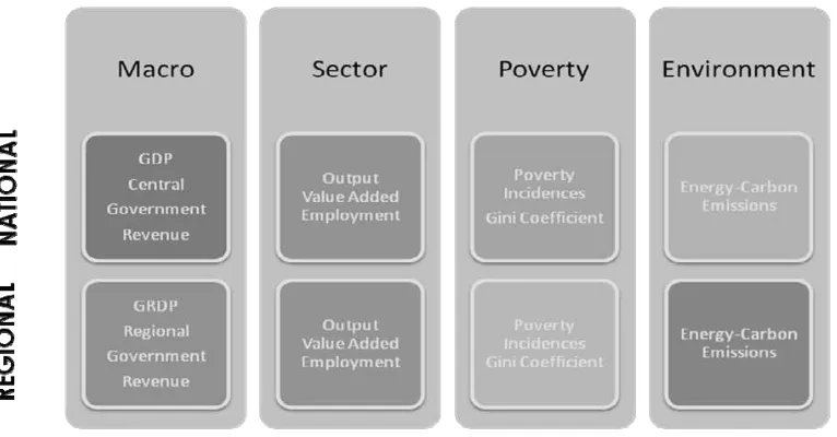
Both rural and urban households in each region are disaggregated using a top-down income-distribution model to become 100 rep-resentative households. CO2 emission from energy use by both production activities and households is modelled, but not that due to deforestation and land conversion. Hence, not only is IRSA-INDONESIA5 able to present the typical macro indicators such as regional gross domestic product (GDP) as well as la-bour and household consumption, but also gini and poverty indexes as well as CO2 emission for each region. Figure 2 summarises indica-tors available in IRSA-INDONESIA5 and which will apply until 2020.

Information capturing all these inter-regional dynamics is available in the 2005 Indonesian inter-regional social accounting matrix (Indonesia IRSAM) developed under the APSI project as well (Resosudarmo, et al.

2009a; 2009b).

3. IRSA-INDONESIA5: Basic Systems of Equation

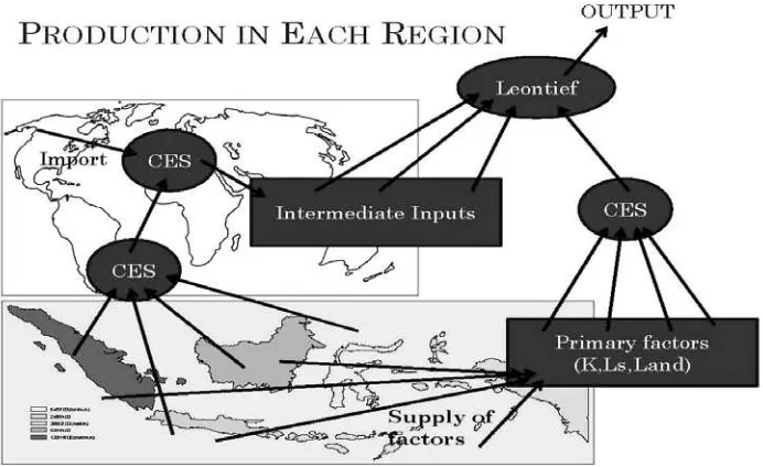
The summary of mathematical equations within IRSA-INDONESIA5 is as follows. On the production side, a nested production func-tion is utilised. At the top level of the produc-tion funcproduc-tion model for each commodity is a Leontief production function between all intermediate goods needed for production and a composite of value added (Figure 3), which is a constant elasticity of substitution (CES) function between capital, labour and land.

(8)

Figure 2. Economic Indicators

(9)

At each level of this nested production function, firms maximise their profits subject to the production function at that level. A zero profit condition is assumed to represent a fully competitive market. Firms then distribute their products domestically and abroad. An export demand function and domestic demand system determines the amount of goods sent abroad or retained for domestic consumption.

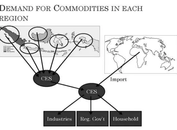
Household demand for each commodity is a Linear Expenditure System (LES) model obtained from a model where households maximise a Stone-Geary utility function sub-ject to a certain budget constraint. Sources of household income are their income from pro-viding labour and capital in production activi-ties in various regions, transfers from national and regional governments, transfers from other households and remittances from abroad (Figure 4). Meanwhile commodities consumed by households (as well as regional government and industries) in each region are a composite of domestic products and imports with a con-stant elasticity of substitution according to the usual Armington function. Composite

domes-tic products are products from various regions which also have a constant elasticity of sub-stitution. The consumption of households, government and industries creates a system of demand functions. (Figure 5).

Household demand equations mentioned above are connected to a top-down income-distributional module which disaggregates each household group (urban and rural house-holds) in each region into 100 household groups. The income of these 100 households is determined by a share parameter distributing the income of the original household. Expen-diture for each of these 100 households is cal-culated using an LES demand function derived from a Stone-Geary utility function.

Market clearing requires that all markets for commodities and factors of production are in a state of equilibrium; i.e. supply matches demand. The inter-temporal part of the model consists mainly of two equations: first, an equation representing capital accumulation from one year to the next; and second, the growth of the country’s labour force.

(10)

Figure 5. Commodity Market

IMPLEMENTATION

This section provides several basic analy-ses utilising IRSA-INDONESIA5. As an ana-lysing tool, it could well illustrate the impact economic policy has on various national and regional economic indicators, such as gross domestic product (GDP), sectoral output, household consumption, the poverty level, income distribution typically represented by the gini index, and CO2 emitted by combus-tion. Figure 6 illustrates the various indicators that IRSA-INDONESIA5 can produce. These economic indicators in general fall into four major categories, namely macroeconomic, sectoral, poverty, and environmental. They are available both at national and regional levels.

IRSA-INDONESIA5 can be utilised to analyse impacts on various national and re-gional economies. For example (Figure 7), the model can illustrate the impact of national policies or international shocks—such as fluctuations in the international oil price, the reduction of import tariffs, and changes in nation-wide indirect taxes or subsidies—on regional economic indicators. On the other

hand, this model can also perform a reverse-causality analysis. In other words, it can be used to analyse nation-wide impacts due to region-specific shocks, such as changes in regional taxes, and regional productivity shocks due to drought, tsunami, or other natu-ral disasters. Lastly, it can also reflect impacts due to changes in national and regional rela-tionships, for example changes in the formula of inter-regional fiscal transfers.

The following sub-sections illustrate more specific implementations of IRSA-INDONESIA5. Several broad different policy simulations are conducted. The period under observation is from 2005 to 2020. To simplify the presentation, only results for 2020 are given. The aim of these simulations is to shed some light on solving the issues of (1) reducing the development gap among regions in the country, (2) achieving low carbon growth and (3) reducing deforestation.

1. Designing Baseline (Sim0)

(11)

needed to act as a benchmark from which to compare all other simulations. The baseline also makes several basic assumptions, the most fundamental one being the assumption that the structure of the economy does not change much during the simulation period. From 2006 until 2010 the GDP grew approxi-mately according to the actual numbers

re-ported by the Indonesian central statistical agency (BPS). For the remaining years up to 2020, GDP growth is assumed to be at ap-proximately 6 percent following the (lower bound) prediction of the Government's Master Plan for Economic Expansion and Accelera-tion 2011-2025.

Figure 7. Economic Indicators

(12)

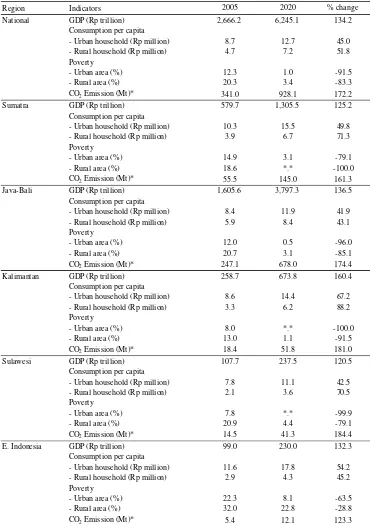
Table 3. Several Indicators in the Baseline Scenarios

Region Indicators 2005 2020 % change

National GDP (Rp trillion) 2,666.2 6,245.1 134.2

Consumption per capita

- Urban household (Rp million) 8.7 12.7 45.0

- Rural household (Rp million) 4.7 7.2 51.8

Poverty

- Urban area (%) 12.3 1.0 -91.5

- Rural area (%) 20.3 3.4 -83.3

CO2 Emission (Mt)* 341.0 928.1 172.2

Sumatra GDP (Rp trillion) 579.7 1,305.5 125.2

Poverty

- Urban area (%) 14.9 3.1 -79.1

- Rural area (%) 18.6 *.* -100.0

CO2 Emission (Mt)* 55.5 145.0 161.3

Java-Bali GDP (Rp trillion) 1,605.6 3,797.3 136.5

Poverty

- Urban area (%) 12.0 0.5 -96.0

- Rural area (%) 20.7 3.1 -85.1

CO2 Emission (Mt)* 247.1 678.0 174.4

Kalimantan GDP (Rp trillion) 258.7 673.8 160.4

Poverty

- Urban area (%) 8.0 *.* -100.0

- Rural area (%) 13.0 1.1 -91.5

CO2 Emission (Mt)* 18.4 51.8 181.0

Sulawesi GDP (Rp trillion) 107.7 237.5 120.5

Poverty

- Urban area (%) 7.8 *.* -99.9

- Rural area (%) 20.9 4.4 -79.1

CO2 Emission (Mt)* 14.5 41.3 184.4

E. Indonesia GDP (Rp trillion) 99.0 230.0 132.3

Poverty

- Urban area (%) 22.3 8.1 -63.5

- Rural area (%) 32.0 22.8 -28.8

CO2 Emission (Mt)* 5.4 12.1 123.3

Note: * = CO2 emission from energy combustion; *.* = a trivial number.

(13)

Table 3 provides several general indica-tors as a result of this baseline scenario. It demonstrates the Indonesian GDP in 2020 will be approximately 134 percent higher than in 2005. Of the Indonesian regions, it is expected that Kalimantan will grow the fastest. Urban poverty at the national level goes down to 1 percent, while rural poverty is 3 percent in 2020. The poverty level in rural Sumatra, ur-ban Java, urur-ban Kalimantan and urur-ban Sulawesi is expected to be zero or close to zero by then. The level of total CO2 emission from energy combustion is predicted to be 172 percent higher than in 2005.

2. Fiscal Decentralisation (Sim1)

A fiscal decentralisation policy simulation scenario is where local governments receive a greater fiscal transfer allocation from the cen-tral government. In this type of policy scenario the central government is asked to increase its fiscal transfer to local governments through a central-to-regional fiscal transfer, which con-sists of four types of fund allocation, i.e. tax revenue shared funds, natural resource revenue shared funds, specific allocation funds (DAK or Dana Alokasi Khusus), and general alloca-tion funds (DAU or Dana Alokasi Umum). Typically, the central government increases its transfers to local governments through the general allocation fund or specific allocation fund. In doing so, the central government could increase each regional government’s budget proportionally to its current budget; or it could increase transfers to each regional government by giving certain amounts of ad-ditional lump-sum funds. The implication is that central government expenditure will be reduced by an equal amount in both scenarios.

The hypothesis of the two policy options above is as follows. When central government expenditure on goods and services is expected to decrease, this tends to have a contractionary effect on the economy through the decline in demand for commodities. On the other hand, after receiving a larger fiscal transfer from the

central government, regional governments will increase their consumption expenditure. This tends to have an expansionary effect on the economy. Whether or not the national demand will decline depends on which force is stronger. The impact on each region also de-pends on the nature of inter-regional trade. The regions that supply a considerable amount of goods and services to the central govern-ment will be more affected.

Another possible scenario (policy option) is that the central government increases its fiscal transfer to some regions, typically the regions that lag behind, and decreases the amount of fiscal transfer to the more advanced regions. The main hypothesis for this policy option is that those regions that lag behind will grow faster and close the development gap among regions in the country. It is important to note that the more advanced regions will be negatively affected and so it is not that clear what the impact of this policy will be on the national economy.

The simulation run for this paper adopts the third option; in this simulation, Eastern Indonesia receives an additional central gov-ernment transfer of 5 percent compared to the base line situation, from 2010 until the end of the simulation year. In this simulation, all the additional budget received by Eastern Indone-sia will be used for consumption expenditures. The consumption pattern of Eastern Indone-sia’s government does not change, just the amount of each expenditure increases. The additional funds for Eastern Indonesia are ac-quired from an equal amount of fiscal transfer reduction for Java-Bali. The main argument for doing this is that Eastern Indonesia is the least developed region in the country and that increased fiscal transfers from the central gov-ernment will enable the region to catch up.

3. Regional Productivity (Sim2)

(14)

can improve due to, among other things, equipment maintenance and the adoption of new technology. Labour productivity can in-crease due to labour quality improvements resulting from better education or new knowl-edge.

In this second simulation it is assumed that the rate of improvement in labour quality in Eastern Indonesia is higher than that of the other islands. Please note that by 2020, labour quality in Eastern Indonesia could still be lower than in the rest of Indonesia. The main reasons for Eastern Indonesia’s faster labour quality growth are that it starts from a lower base, there is a movement of labour with higher skills into the area and the quality of education in the area is improved. Better la-bour quality, in turn, translates, in this paper, into an increase in both labour and capital pro-ductivity by as much as 1 percent higher than the baseline between 2010 and the end of the simulation year.

With this acceleration of labour and capi-tal productivity it is expected that Eastern In-donesia will develop faster than it would under the baseline scenario and this will benefit the nation as a whole in terms of poverty reduc-tion and higher growth.

4. Energy Efficiency (Sim3)

With increasing global concern regarding climate change, adaptation and mitigation strategies become very important. Indonesia faces a variety of climate change impacts, from sea-level rise to a changing hydrological cycle and more frequent droughts and floods, to greater stresses on public health. These will require attention and corrective action if de-velopment is to be safeguarded in the face of changes in the natural world. Indonesia itself is a significant emitter of greenhouse gases, especially connected to deforestation. How-ever, reducing these emissions creates its own challenges; particularly in calculating how these activities will affect the economy and the people.

The third simulation relates to the im-provement in efficiency of energy use. There are many forms energy efficiency can take, albeit mostly related to maintenance and tech-nological improvements. Energy efficiency can also occur both in the private and indus-trial sectors. Households deciding to use more energy efficient light bulbs and heaters is an example of private sector energy efficiency. Energy efficiency in the industrial sector mainly relates to capital, specifically equip-ment. Equipment maintenance and technologi-cal improvements are examples of how energy efficiency can be achieved in this sector.

Note that the industrial sector itself con-sists of many smaller sectors, such as food and beverage, cement, basic metal, rubber, and others. As such, energy efficiency in the in-dustrial sector does not necessarily mean an increase in efficiency for all sectors at once. Implementation of IRSA-INDONESIA5 can simulate an increase in energy efficiency in all sectors at once or selected sectors only. Fur-thermore, in some cases, energy efficiency involves additional costs, e.g. through the adoption of new energy efficient technology acquired from abroad which the government can subsidise or, alternately for which the in-dustrial sector bears the entire cost.

There is an instance in the simulation run in this paper where the stimulus occurs from equipment maintenance and technological improvements. The simulation looks at the impact of a gradual improvement in energy efficiency of up to 10 percent by 2015, begin-ning in 2010, in the food processing, textile, rubber, cement, basic metal and pulp and pa-per industries; i.e. the energy intensive indus-tries.

(15)

heavily on their energy sectors, particularly Kalimantan, will be negatively affected. Meanwhile regions where food processing, textile, rubber, cement, basic metal and pulp and paper industries are mostly located, par-ticularly Java, will be positively affected.

5. Electricity Sector (Sim4)

This simulation concerns how electricity has been generated. It investigates what the impact on the economy would be if the elec-tricity sector were to be more efficient in util-ising energy inputs to produce electricity. First, electricity could be cheaper and so in-duce higher economic growth. Second, CO2 emissions could be lower, in particular, since most coal is utilised by the electricity power generating sector rather than by other sectors.

In this simulation, it is assumed that the electricity sector becomes gradually more effi-cient in using fossil fuels. It becomes 20 per-cent more efficient between 2010 and 2015. It is assumed in this simulation that there is no significant cost associated with the improve-ment. In other words, such costs are taken care of exogenously. In general this situation will improve the economic performance of all re-gions.

6. Energy Subsidy Policy (Sim5)

Subsidies have always been an important instrument for the Indonesian government. This issue generally relates to the question of who benefits the most from a government subsidy—certainly an important issue as it has direct bearing on the purpose of a subsidy. Of course, there are many types of subsidies, ranging from direct government transfers to low-income households to industrial subsidies to help reduce production costs in a certain sector.

This simulation, however, does not inves-tigate the impacts of implementing a subsidy. Instead it looks at the impacts of reducing fuel subsidies. In other words, the fifth simulation

looks at the gradual elimination of fuel subsi-dies from the year 2010 until its full abolition in 2015. The entire financial gain from subsidy reduction is distributed back into the economy through government spending. It is hard to predict what impact this will have on the economy. In general the economy might per-form better compared to the baseline, but this will probably not be the case in all regions.

7. Carbon Tax (Sim6)

In this simulation, it is assumed there is a carbon tax of as much as Rp.10,000 per ton of CO2 from 2010 onwards. This carbon tax revenue enables the government to spend more on goods and services. It is expected that industries using highly polluting energy, such as coal, will be negatively affected. On the other hand increasing the government budget will create the stimulus to boost the economy. It remains to be seen which force is stronger.

8. Deforestation (Sim7)

In this simulation, deforestation outside Java-Bali is assumed to be reduced by 10 per-cent from 2012 onwards mainly due to effec-tive control of logging activities; i.e. the amount of logs produced is controlled so as to decline by as much as 10 percent from the baseline condition. Here, no compensation is offered. In a way, this simulation can also be a benchmark for comparison in other simula-tions related to reducing the rate of deforesta-tion, specifically cases involving carbon emis-sion reduction compensation.

(16)

OBSERVATIONS REGARDING RESULTS

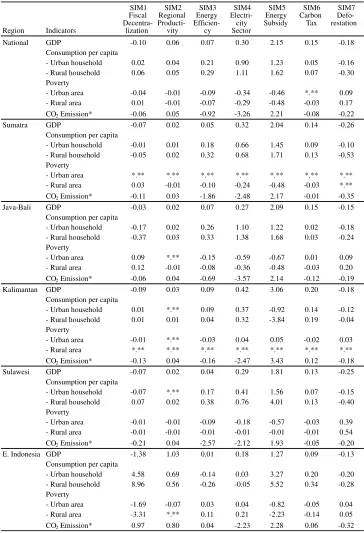
The following sections look at the results of simulations mentioned above. They com-pare four economic indicators, namely gross domestic product (GDP), household con-sumption per capita, poverty, and carbon emission, for all the simulations with respect to the baseline simulation (Table 4). All num-bers are percentage changes; i.e. results from the policy simulations divided by the baseline minus one multiplied by a hundred, except for poverty. Poverty is the difference between poverty outcomes from the policy simulation and the baseline situation.

GDP is the most common measure of re-gional economic performance. A higher GDP indicates higher welfare in the region. The indicator that most specifically measures household welfare is household consumption per capita. It is assumed that the more a household consumes, the better off it is. This is the indicator typically used to differentiate rural and urban households. Even when rural and urban households are affected similarly, whether positively or negatively, in many cases, magnitudes of the impact do differ.

Concerning the poverty indicator, the most common parameter is the head-count poverty index. This index shows the percen-tage of poor people in a certain region; i.e. those living below a certain poverty line. The World Bank commonly use $1 a day or $2 a day as the poverty line. BPS produces a pov-erty line for each province in Indonesia each year. In 2008, the poverty line for urban areas was slightly above Rp. 200,000 per capita per month and slightly below Rp. 200,000 per capita per month for rural areas. This work will use the poverty lines produced by BPS and so the poverty indicators show the per-centage of poor people based on their defini-tions.

CO2 emission indicators represent the total emission from fuel combustion activities per year. As mentioned before, these numbers exclude the amount of emission from

defores-tation, land use and other factors.

In observing the results of the simulation, it is important to note that this paper assumes that the structure of the economy, except for the shocks introduced in each policy simula-tion, remains the same during the period of the simulation. The main benefit of having this assumption is that it can be sure that the re-sults of this paper are mainly due to the shocks introduced. The drawback is that this might never happen in the real world. Any shock will always change the structure of the economy. Hence, in a way, this paper underestimates the "full" impact of each policy simulation.

1. Fiscal Decentralisation (Sim1)

The results of this simulation can be seen in column SIM1 of Table 4. The initial intui-tion is that increased central government trans-fers to Eastern Indonesia will benefit the region; i.e. The Eastern Indonesian economy under this policy will be better than the base-line scenario. However, this policy might negatively affect the region, in this case Java-Bali, which receives a lesser fiscal transfer from the central government. Since the initial condition is that the economy of Java-Bali performs better than that of Eastern Indonesia, the policy of increasing the fiscal transfer will lower the gap between Eastern Indonesia and Java-Bali.

(17)

Table 4. Simulation Results in 2020 as Compared to the Baseline (in %)

SIM1 SIM2 SIM3 SIM4 SIM5 SIM6 SIM7

Region Indicators

Fiscal

Decentra-lization

Regional

Producti-vity

Energy Efficien-cy

Electri-city Sector

Energy Subsidy

Carbon Tax

Defo-restation

National GDP -0.10 0.06 0.07 0.30 2.15 0.15 -0.18

- Urban household 0.02 0.04 0.21 0.90 1.23 0.05 -0.16 - Rural household 0.06 0.05 0.29 1.11 1.62 0.07 -0.30 Poverty

- Urban area -0.04 -0.01 -0.09 -0.34 -0.46 *.** 0.09 - Rural area 0.01 -0.01 -0.07 -0.29 -0.48 -0.03 0.17 CO2 Emission* -0.06 0.05 -0.92 -3.26 2.21 -0.08 -0.22

Sumatra GDP -0.07 0.02 0.05 0.32 2.04 0.14 -0.26

- Urban household -0.01 0.01 0.18 0.66 1.45 0.09 -0.10 - Rural household -0.05 0.02 0.32 0.68 1.71 0.13 -0.53 Poverty

- Urban area *.** *.** *.** *.** *.** *.** *.**

- Rural area 0.03 -0.01 -0.10 -0.24 -0.48 -0.03 *.** CO2 Emission* -0.11 0.03 -1.86 -2.48 2.17 -0.01 -0.35

Java-Bali GDP -0.03 0.02 0.07 0.27 2.09 0.15 -0.15

- Urban household -0.17 0.02 0.26 1.10 1.22 0.02 -0.18 - Rural household -0.37 0.03 0.33 1.38 1.68 0.03 -0.24 Poverty

- Urban area 0.09 *.** -0.15 -0.59 -0.67 0.01 0.09 - Rural area 0.12 -0.01 -0.08 -0.36 -0.48 -0.03 0.20 CO2 Emission* -0.06 0.04 -0.69 -3.57 2.14 -0.12 -0.19

Kalimantan GDP -0.09 0.03 0.09 0.42 3.06 0.20 -0.18

- Urban household 0.01 *.** 0.09 0.37 -0.92 0.14 -0.12 - Rural household 0.01 0.01 0.04 0.32 -3.84 0.19 -0.04 Poverty

- Urban area -0.01 *.** -0.03 0.04 0.05 -0.02 0.03

- Rural area *.** *.** *.** *.** *.** *.** *.**

CO2 Emission* -0.13 0.04 -0.16 -2.47 3.43 0.12 -0.18

Sulawesi GDP -0.07 0.02 0.04 0.29 1.81 0.13 -0.25

- Urban household -0.07 *.** 0.17 0.41 1.56 0.07 -0.15 - Rural household 0.07 0.02 0.38 0.76 4.01 0.13 -0.40 Poverty

- Urban area -0.01 -0.01 -0.09 -0.18 -0.57 -0.03 0.39 - Rural area -0.01 -0.01 -0.01 -0.01 -0.01 -0.01 0.54 CO2 Emission* -0.21 0.04 -2.57 -2.12 1.93 -0.05 -0.20

E. Indonesia GDP -1.38 1.03 0.01 0.18 1.27 0.09 -0.13

- Urban household 4.58 0.69 -0.14 0.03 3.27 0.20 -0.20 - Rural household 8.96 0.56 -0.26 -0.05 5.52 0.34 -0.28 Poverty

- Urban area -1.69 -0.07 0.03 0.04 -0.82 -0.05 0.04 - Rural area -3.31 *.** 0.11 0.21 -2.23 -0.14 0.05 CO2 Emission* 0.97 0.80 0.04 -2.23 2.28 0.06 -0.32

Note: * = CO2 emission from energy combustion; *.** = a trivial number.

(18)

Regarding household consumption per capita, it can be seen that Eastern Indonesia is the only region likely to benefit from an in-creased transfer of funding to the region. The household consumption per capita in the re-gion increases by almost 9 in percent urban areas and 5 percent in rural areas, compared to the situation under baseline conditions. This higher household consumption per capita is translated into a lower level of poverty by as much as 3 and 2 percent in urban and rural areas, respectively.

Household consumption per capita does not change much in other regions. In this simulation Java-Bali faces a lower transfer of funding from the central government com-pared to the baseline situation, and so it is natural that household consumption per capita in this region is affected the most negatively. A lower household consumption per capita is then translated into a higher poverty level in this region. Observing what is happening in the Eastern Indonesian and Java-Bali regions, it can be concluded that shifting funding from rich to poor regions does work in reducing the poverty level of poor regions.

2. Regional Productivity (Sim2)

In this scenario, productivity in Eastern Indonesia alone improves faster and induces a higher GDP for Eastern Indonesia in 2020 than it does under baseline conditions. Better productivity also induces a higher consump-tion per capita in rural and urban areas in these regions, and translates into a lower level of poverty. In rural areas, however, the change in the poverty level is minimal.

The other regions also benefit from a more productive Eastern Indonesia as their GDPs in 2020 are also slightly higher in this scenario compared to the baseline. Nevertheless the impacts on other regions’ GDPs are not that great and so household consumption per capita in other regions is only marginally higher than the baseline situation. Poverty levels in rural and urban Sulawesi, rural Java-Bali and rural

Sumatra in 2020 are lower than their baseline levels.

It can be seen in this scenario that produc-tivity improvement achieves both the targets of higher national economic growth and duction in the development gap between re-gions. Given this result, there is certainly room for the government to incur “extra” costs to ensure the improvement of productivity such as by improving the educational system in less developed regions.

3. Energy Efficiency (Sim3)

More efficient use of energy in the energy intensive sectors—i.e. food processing, textile, rubber, cement, basic metal and pulp and pa-per industries—is expected to lower the op-eration costs of those sectors, and enable them to sell their products at a lower price. This generates higher demand for the products of those sectors and so induces higher returns to factor inputs including incomes of workers who work in those sectors. These higher re-turns potentially improve household con-sumption so households will be able to spend more, with the outcome that the economy is expected to grow. On the other hand, more efficient use of energy reduces demand for energy products meaning lower returns to factor inputs in the energy sectors including work income. Ultimately, these lower incomes could potentially reduce the economy. Hence, more efficient energy usage could have a positive or negative effect on the economy.

(19)

long-run are higher than the negative impact of a lower demand for energy in the short-run.

In this scenario, household consumption per capita in general is higher than the baseline scenario in all regions. This higher income per capita is translated into a lower level of pov-erty in most regions, except for urban Sumatra and rural Kalimantan. In those areas, the levels of poverty remain the same as under baseline conditions.

Under this scenario CO2 emission from energy combustion in 2020 is lower than the baseline, representing lower consumption of fuels. The ability to improve energy efficiency in the energy intensive sectors not only creates higher growth, but also reduces CO2 emission from energy combustion, demonstrating that this is certainly one way to control CO2 emis-sion. Since the economy would benefit from this improvement, there is a room for the gov-ernment to create programs or incentives to ensure this improvement in energy efficiency.

4. Electricity Sector (Sim4)

A more efficient electricity sector makes it cheaper to produce electricity. The lower price of electricity lowers costs in all other sectors except for the primary energy sector. House-holds will also be able to consume more goods and services other than electricity. The overall potential impact is the economy becoming larger than the baseline situation. On the other hand, due to a more efficient electricity sector, primary energy sectors might decline and so potentially negatively affect the economy. Ultimately it remains to be seen whether or not a more efficient electricity sector benefits the economy.

Column SIM4 in Table 4 shows that it turns out that a more efficient electricity sector does induce higher GDPs in all regions by 2020 compared to the baseline situation. The benefits of having a more efficient electricity sector are greater than the negative impact due to the decline in the primary energy sector. As

GDPs increase, household consumption per capita in both rural and urban areas in all re-gions increases as well, except in rural Eastern Indonesia. Poverty, except in Papua and Kali-mantan, declines. In Papua and KaliKali-mantan, the increasing poverty is due to the increase in income of relatively rich households, while it declines somewhat in the case of relatively poor households.

In terms of CO2 emissions from energy combustion, a more efficient electricity sector is an effective way to reduce these emissions. It is argued that it is even more effective than more efficient energy use in energy intensive industries. The main reason for this is that coal, the dirtiest of all energy sources in terms of CO2 emission, is mostly consumed by the electricity sector, whereas the energy intensive industries use various types of energy. It is important to note as well that in terms of policy implementation, it is probably easier to improve the efficiency of the electricity sector, since there are fewer electric power generators than energy intensive industries.

5. Energy Subsidy Policy (Sim5)

It is important to note that currently the energy subsidy is for gasoline and kerosene. This subsidy should be eliminated for the sim-ple reason that it encourages inefficient use of energy. A more sophisticated reason is that this inefficient use of energy leads to a state of equilibrium of goods and services in which society will not achieve the maximum possible benefits. Eliminating this subsidy should in-crease the GDP of the country. Column SIM5 in Table 4 illustrates this situation; compared to one baseline conditions GDP for 2020 in-creases in all regions. And in general, a higher GDP leads to an increase in household con-sumption per capita and a reduction of pov-erty.

(20)

compared to the change in GDP of other re-gions in 2020 under this scenario and at base-line, the change in Kalimantan is the highest. However, firstly, this is not true for the changes in household consumption per capita; i.e. the changes in household consumption per capita in Kalimantan are, in general, not higher than those in other regions, except in Papua. Considerable GDP gains go to an in-crease in return to capitals in the region com-pared to other regions. This means that indus-tries in Kalimantan tend to be capital intensive ones. The second issue concerning Kalimantan is that an increase in household consumption per capita is not automatically translated into a reduction of poverty. Capital intensive indus-tries tend to employ more highly skilled work-ers, and so when the size of the economy increases—i.e. the capital intensive industries expand—it is mostly the skilled workers, who are relatively not poor, who receive a higher income. The impact of this economic expan-sion on the poor is relatively small.

The elimination of an energy subsidy does not always lead to lower CO2 emission for several reasons. First, elimination of gasoline and kerosene subsidies could lead to greater use of coal which emits more CO2 than gaso-line and kerosene. Second, the elimination of an energy subsidy might lead to a reduction in the use of energy and so less CO2 would be emitted in the short run. In the long-run, since the economy grows faster without the energy subsidy, the economy will consume more en-ergy. But energy intensity (energy use per unit of GDP) remains lower under the elimination of the subsidy compared to the situation with-out energy subsidy elimination. Simulation in this work demonstrates the second case. In the short run, CO2 declines, but not in the long run, since the economy grew faster than in the baseline situation.

6. Carbon Tax (Sim6)

A carbon tax per ton of CO2 makes a dirty type of energy relatively more expensive.

Un-der such conditions coal would become rela-tively more expensive, and gas and renewable energy sources relatively cheaper. A carbon tax in general makes it more costly to produce products and so potentially negatively affects the economy. However, in this scenario, the whole revenue from carbon tax is redistributed to the economy by increasing government spending. This spending should positively affect the economy. Therefore, whichever force is bigger (the negative or the positive force) will determine the overall impact of a carbon tax on the economy.

Column SIM6 in Table 4 shows that a carbon tax, overall, positively affects the economy. GDPs in all regions in 2020 are higher than the baseline. The level of CO2 emission in 2020 is also lower than the condi-tions. It is important to note that when the car-bon tax is initially implemented, the level of CO2 emission is much lower than in the base-line scenario. How low it is depends on whether or not the model allows a substitution of dirty sources for cleaner sources of energy. Nevertheless, since the economy under a car-bon tax grew faster than it did without one, the gap of CO2 emission between these two sce-narios is reduced. Eventually the total CO2 emission under a carbon tax will be higher than it is without one, since the economy is much larger. However, carbon emission inten-sity will still be lower under a carbon tax than under the baseline situation.

(21)

7. Deforestation (Sim7)

When less timber extraction is allowed from off-Java islands, the national GDP in 2020 is lower than the baseline scenario. In terms of GDP, Sumatra and Kalimantan are affected the most. This is natural since most timber comes from these two islands and so a 10 percent reduction is significant for them. What is rather surprising is the result for Java-Bali. Although it does not have much remain-ing forest and moreover no restrictions on har-vesting timber, the region is negatively af-fected. The main reason for this is that major-ity of wood processing industries are in Java and they are affected when less wood is avail-able. As a consequence of this lower GDP, both urban and rural household consumption per capita in all regions in 2020 is lower than at baseline, and urban and rural poverty levels in all regions are higher.

This simulation indicates that people do need compensations for timber harvesting re-strictions. The compensations should not only be distributed to rural people (i.e. forest com-munities) in forest production regions, but also to urban people in those regions and to also to the people in Java-Bali.

CONCLUSIONS

This paper aims to introduce IRSA-INDONESIA5 which was developed under the Analysing Path of Sustainable Indonesia (APSI) project as a policy tool for the Indone-sian government. IRSA-INDONESIA5 is a dynamic inter-regional CGE. This paper also shows how this model can be implemented to help resolve several problems faced by Indo-nesia. Here are several general lessons from the implementation of IRSA-INDONESIA5 with regard to the issues of (1) reducing the development gap among regions in the coun-try, (2) achieving low carbon growth and (3) reducing deforestation. Furthermore detailed research is needed to achieve more detailed policy lessons.

Reducing the development gap and en-hancing national economic growth: SIM1 and SIM2 reveal that the best way to reduce the development gap among regions is by creating effective programs to accelerate the growth of human capital in the less developed regions. This way, they will grow faster and spread to other regions so that ultimately the whole country will grow faster.

There are certainly some rooms to reallo-cate the transfers from the central to regional governments in favour of less developed re-gions. However, this policy should be exe-cuted cautiously so that the negative impact on other regions is relatively small.

Achieving low carbon and high economic growth: In the short-term, the elimination of energy subsidies and/or implementation of a carbon tax works well in reducing CO2 emis-sion and producing higher economic growth. Such measures can be implemented gradually. For instance, the rate of a carbon tax can be initially low and then gradually be increased.

In the long-run, however, technological improvement, particularly toward a more en-ergy efficient technology, is needed to main-tain a relatively low level of emission with continued high growth. For Indonesia, the first step is to improve the efficiency of energy use in the electricity sector. The second step is to force the energy intensive industries to be more efficient in using energy, and eventually all industries as well as households. Techno-logical improvement, if available, can be ef-fective in achieving lower CO2 emission while encouraging the economy to grow faster. Hence, the government should consider in-vesting in programs that ensure the transfer of more energy efficient technology to the coun-try.

(22)

there are two ways of utilising this compensa-tion. Firstly it could be distributed to house-holds. It is important to note that this compen-sation should not only be given to forest com-munities, but also to the poor in urban areas and regions where wood processing industries are located. The compensation funding is ex-pected to compensate for income lost due to the reduced activity of the logging and wood processing industries. If households receive more income, it is also expected that house-hold consumption will encourage the economy to grow faster.

Secondly, the deforestation compensation could be distributed to the government, in-cluding regional governments, with two aims in mind. First, it is expected that with this funding the government could create effective reforestation programs or improve the forest industry areas that are currently inefficient, so that reduced deforestation can be achieved without any or only a marginal reduction in logging. Second, the government would be able to spend more on various goods and ser-vices and so encourage the economy to grow, compensating for the decline due to a reduc-tion in timber harvesting. It is important to note that combinations of the various options mentioned above are certainly possible and are to be encouraged so that the maximum bene-fits from deforestation compensation can be achieved.

REFERENCES

Abimanyu, A, 2000. “Impact of Agriculture Trade and Subsidy Policy on the Macroeconomy, Distribution, and Envi-ronment in Indonesia: A Strategy for Fu-ture Industrial Development.” The Devel-oping Economies, 38(4), 547–571.

Alm, J., R.H. Aten, and R. Bahl, 2001. “Can Indonesia Decentralise Successfully? Plans, Problems and Prospects.” Bulletin of Indonesian Economic Studies, 37(1), 83-102.

Azis, I.J., 2000. “Modelling the Transition from Financial Crisis to Social Crisis”.

Asian Economic Journal, 14(4), 357-387. Behrman, J.R., J.D. Lewis, and S. Lofti, 1989.

“The Impact of Commodity Price Insta-bility: Experiments with A General Equi-librium Model for Indonesia.” In L. R. Klein and J. Marquez. Economics in Theory and Practice: An Eclectic Approach, (eds). 59–100. Dordrecht: Kluwer Academic Publisher.

Central Bureau of Statistics, Institute of Social Studies, and Center for World Food Stud-ies (BPS, ISS, and CWFS), 1986. Report on Modelling: The Indonesian Social Ac-counting Matrix and Static Disaggregated Model. Jakarta: Central Bureau of Statis-tics.

Central Statistical Agency (BPS or Badan Pusat Statistik), 2008. Statistical Year Book of Indonesia 2008. Jakarta: Central Bureau of Statistics.

Dixon, P., B.R. Parmenter, J. Sutton, and D.P. Vincent, 1982. ORANI: A Multisectoral Model of the Australian Economy. Contri-butions to Economic Analysis 142, North-Holland Publishing Company.

Ezaki, M., 1989. “Oil Price Declines and Structural Adjustment Policies in Indone-sia: A Static CGE Analysis for 1980 and 1985”. The Philippine Review of Eco-nomics and Business, 26(2), 173- 207. Hill, H., B.P. Resosudarmo, and Y.

Vidyat-tama, 2008. “Indonesia's Changing Eco-nomic Geography”. Bulletin of Indonesian Economic Studies, 44(3), 407-435.

Lewis, J.D., 1991. “A Computable General Equilibrium (CGE) Model of Indonesia.” HIID’s series of Development Discussion Papers No. 378, Harvard University. Pambudi, D., and A.A. Parewangi, 2004.

(23)

Resosudarmo, B.P., 2002. “Indonesia’s Clean Air Program.” Bulletin of Indonesian Economic Studies, 38 (3), 343–365.

Resosudarmo, B.P. (ed.), 2005. The Politics and Economics of Indonesia Natural Re-sources. Singapore: Institute for Southeast Asian Studies.

Resosudarmo, B.P., 2008. “The Economy-wide Impact of Integrated Pest Manage-ment in Indonesia.” ASEAN Economic Bulletin, 25(3), 316–333.

Resosudarmo, B.P., A.A. Yusuf, D.A. Nurdi-anto, and D. Hartono, 2009. “Regional Economic Modelling for Indonesia of the IRSA-INDONESIA5.” Working Papers in Trade and Development, Working Paper No. 2009/21, The Arndt-Corden Division of Economics, ANU College of Asia and the Pacific.

Resosudarmo, B.P., D. Hartono, and D.A. Nurdianto, 2009a. “Inter-Island Economic Linkages and Connections in Indonesia.”

Economics and Finance Indonesia, 56(3), 297-327.

Resosudarmo, B.P., D.A. Nurdianto, and D. Hartono, 2009b. “The Indonesian Inter-Regional Social Accounting Matrix for Fiscal Decentralisation Analysis.” Journal of Indonesian Economy and Business,

24(2), 145 - 162.

Resosudarmo, B.P. and F. Jotzo (eds.), 2009.

Working with Nature against Poverty: Development, Resources and the

Environ-ment in Eastern Indonesia. Singapore: In-stitute for Southeast Asian Studies.

Resosudarmo, B.P., L.E. Wuryanto, G.J.D. Hewings, and L. Saunders, 1999. “Decen-tralization and Income Distribution in the Inter-Regional Indonesian Economy.” In G.J.D. Hewings, M. Sonis, M. Madden and Y. Kimura, Advances in Spatial Sciences: Understanding and Interpreting Economic Structure, (eds), 297-315, Germany: Springer-Verlag.

Resosudarmo, B.P. and Y. Vidyattama, 2006. “Regional Income Disparity in Indonesia: A Panel Data Analysis.” ASEAN Eco-nomic Bulletin, 23(1), 31-44.

Resosudarmo, B.P. and Y. Vidyattama, 2007. “East Asian Experience: Indonesia”, in

The Dynamics of Regional Development: The Philippines in East Asia, A.M. Balisacan and H. Hill (eds.), Cheltenham Glos. England: Edward Elgar, 123-153. Thorbecke, T., 1991. “Adjustment, Growth

and Income Distribution in Indonesia.”

World Development, 19(11), 1595-1614. Warr, P., 2005. “Food Policy and Poverty in

Indonesia: A General Equilibrium Analy-sis.” The Australian Journal of Agricul-tural and Resource Economics, 49, 429– 451.