Getting Started
with
25 Recipes for Getting
Started with R
Paul Teetor
25 Recipes for Getting Started with R by Paul Teetor
Copyright © 2011 Paul Teetor. All rights reserved. Printed in the United States of America.
Published by O’Reilly Media, Inc., 1005 Gravenstein Highway North, Sebastopol, CA 95472. O’Reilly books may be purchased for educational, business, or sales promotional use. Online editions are also available for most titles (http://my.safaribooksonline.com). For more information, contact our corporate/institutional sales department: (800) 998-9938 or [email protected].
Editor: Mike Loukides
Production Editor: Adam Zaremba
Proofreader: Adam Zaremba
Cover Designer: Karen Montgomery
Interior Designer: David Futato
Illustrator: Robert Romano
Printing History:
February 2011: First Edition.
Nutshell Handbook, the Nutshell Handbook logo, and the O’Reilly logo are registered trademarks of O’Reilly Media, Inc. 25 Recipes for Getting Started with R, the image of a harpy eagle, and related trade dress are trademarks of O’Reilly Media, Inc.
Many of the designations used by manufacturers and sellers to distinguish their products are claimed as trademarks. Where those designations appear in this book, and O’Reilly Media, Inc. was aware of a trademark claim, the designations have been printed in caps or initial caps.
While every precaution has been taken in the preparation of this book, the publisher and authors assume no responsibility for errors or omissions, or for damages resulting from the use of the information con-tained herein.
Table of Contents
Preface . . . vii
The Recipes . . . 1
1.1 Downloading and Installing R 1
1.2 Getting Help on a Function 3
1.3 Viewing the Supplied Documentation 4
1.4 Searching the Web for Help 6
1.5 Reading Tabular Datafiles 8
1.6 Reading from CSV Files 10
1.7 Creating a Vector 12
1.8 Computing Basic Statistics 13
1.9 Initializing a Data Frame from Column Data 16
1.10 Selecting Data Frame Columns by Position 17
1.11 Selecting Data Frame Columns by Name 21
1.12 Forming a Confidence Interval for a Mean 22
1.13 Forming a Confidence Interval for a Proportion 23
1.14 Comparing the Means of Two Samples 24
1.15 Testing a Correlation for Significance 26
1.16 Creating a Scatter Plot 28
1.17 Creating a Bar Chart 29
1.18 Creating a Box Plot 30
1.19 Creating a Histogram 32
1.20 Performing Simple Linear Regression 33
1.21 Performing Multiple Linear Regression 34
1.22 Getting Regression Statistics 36
1.23 Diagnosing a Linear Regression 39
1.24 Predicting New Values 42
1.25 Accessing the Functions in a Package 43
Preface
R is a powerful tool for statistics, graphics, and statistical programming. It is used by tens of thousands of people daily to perform serious statistical analyses. It is a free, open source system whose implementation is the collective accomplishment of many intel-ligent, hard-working people. There are more than 2,000 available add-ons, and R is a serious rival to all commercial statistical packages.
But R can be frustrating. It’s not obvious how to accomplish many tasks, even simple ones. The simple tasks are easy once you know how, yet figuring out the “how” can be maddening.
This is a book of how-to recipes for beginners, each of which solves a specific problem. The recipe includes a quick introduction to the solution, followed by a discussion that aims to unpack the solution and give you some insight into how it works. I know these recipes are useful and I know they work because I use them myself.
Most recipes use one or two R functions to solve the stated problem. It’s important to remember that I do not describe the functions in detail; rather, I describe just enough to get the job done. Nearly every such function has additional capabilities beyond those described here, and some of those capabilities are amazing. I strongly urge you to read the function’s help page. You will likely learn something valuable.
The book is not a tutorial on R, although you will learn something by studying the recipes. The book is not an introduction to statistics, either. The recipes assume that you are familiar with the underlying statistical procedure, if any, and just want to know how it’s done in R.
These recipes were taken from my R Cookbook (O’Reilly). The Cookbook contains over 200 recipes that you will find useful when you move beyond the basics of R.
Other Resources
I can recommend several other resources for R beginners:
An Introduction to R (Network Theory Limited)
This book by William N. Venables, et al., covers many general topics, including statistics, graphics, and programming. You can download the free PDF book; or, better yet, buy the printed copy because the profits are donated to the R project.
R in a Nutshell (O’Reilly)
Joseph Adler’s book is the tutorial and reference you’ll keep by your side. It covers many topics, from introductory material to advanced techniques.
Using R for Introductory Statistics (Chapman & Hall/CRC)
A good choice for learning R and statistics together by John Verzani. The book teaches statistical concepts together with the skills needed to apply them using R. The R community has also produced many tutorials and introductions, especially in specialized topics. Most of this material is available on the Web, so I suggest searching there when you have a specific need (as in Recipe 1.4).
The R project website keeps an extensive bibliography of books related to R, both for beginning and advanced users.
Downloading Additional Packages
The R project has over 2,000 packages that you can download to augment the standard distribution with additional capabilities. You might see such packages mentioned in the See Also section of a recipe, or you might discover one while searching the Web. Most packages are available through the Comprehensive R Archive Network (CRAN)
at http://cran.r-project.org. From the CRAN home page, click on Packages to see the
name and a brief description of every available package. Click on a package name to see more information, including the package documentation.
Downloading and installing a package is simple via the install.packages function. You would install the zoo package this way, for example:
> install.packages("zoo")
Software and Platform Notes
The base distribution of R has frequent, planned releases, but the language definition and core implementation are stable. The recipes in this book should work with any recent release of the base distribution.
One recipe has platform-specific considerations (Recipe 1.1). As far as I know, all other recipes will work on all three major platforms for R: Windows, OS X, and Linux/Unix.
Conventions Used in This Book
The following typographical conventions are used in this book:
Italic
Indicates new terms, URLs, email addresses, filenames, and file extensions. Constant width
Used for program listings, as well as within paragraphs to refer to program elements such as variable or function names, databases, data types, environment variables, statements, and keywords.
Constant width bold
Shows commands or other text that should be typed literally by the user. Constant width italic
Shows text that should be replaced with user-supplied values or by values deter-mined by context.
This icon signifies a tip, suggestion, or general note.
This icon indicates a warning or caution.
Using Code Examples
This book is here to help you get your job done. In general, you may use the code in this book in your programs and documentation. You do not need to contact us for permission unless you’re reproducing a significant portion of the code. For example, writing a program that uses several chunks of code from this book does not require permission. Selling or distributing a CD-ROM of examples from O’Reilly books does require permission. Answering a question by citing this book and quoting example
code does not require permission. Incorporating a significant amount of example code from this book into your product’s documentation does require permission.
We appreciate, but do not require, attribution. An attribution usually includes the title, author, publisher, and ISBN. For example: “25 Recipes for Getting Started with R by Paul Teetor (O’Reilly). Copyright 2011 Paul Teetor, 978-1-449-30323-5.”
If you feel your use of code examples falls outside fair use or the permission given above, feel free to contact us at [email protected].
Safari® Books Online
Safari Books Online is an on-demand digital library that lets you easily search over 7,500 technology and creative reference books and videos to find the answers you need quickly.
With a subscription, you can read any page and watch any video from our library online. Read books on your cell phone and mobile devices. Access new titles before they are available for print, and get exclusive access to manuscripts in development and post feedback for the authors. Copy and paste code samples, organize your favorites, down-load chapters, bookmark key sections, create notes, print out pages, and benefit from tons of other time-saving features.
O’Reilly Media has uploaded this book to the Safari Books Online service. To have full digital access to this book and others on similar topics from O’Reilly and other pub-lishers, sign up for free at http://my.safaribooksonline.com.
How to Contact Us
Please address comments and questions concerning this book to the publisher: O’Reilly Media, Inc.
1005 Gravenstein Highway North Sebastopol, CA 95472
800-998-9938 (in the United States or Canada) 707-829-0515 (international or local)
707-829-0104 (fax)
We have a web page for this book, where we list errata, examples, and any additional information. You can access this page at:
http://www.oreilly.com/catalog/9781449303235
To comment or ask technical questions about this book, send email to:
For more information about our books, courses, conferences, and news, see our website
at http://oreilly.com.
Find us on Facebook: http://facebook.com/oreilly
Follow us on Twitter: http://twitter.com/oreillymedia
Watch us on YouTube: http://www.youtube.com/oreillymedia
The Recipes
1.1 Downloading and Installing R
Problem
You want to install R on your computer.
Solution
Windows and OS X users can download R from CRAN, the Comprehensive R Archive Network. Linux and Unix users can install R packages using their package management tool.
Windows
• Open http://www.r-project.org/ in your browser.
• Click on “CRAN”. You’ll see a list of mirror sites, organized by country. • Select a site near you.
• Click on “Windows” under “Download and Install R”. • Click on “base”.
• Click on the link to download the latest version of R (an .exe file).
• When the download completes, double-click the .exe file and answer the usual questions.
OS X
• Open http://www.r-project.org/ in your browser.
• Click on “CRAN”. You’ll see a list of mirror sites, organized by country. • Select a site near you.
• Click on “MacOS X”.
• Click on the .pkg file for the latest version of R, under “Files:”, to download it. • When the download completes, double-click the .pkg file and answer the usual
questions.
Linux or Unix
The major Linux distributions have packages for installing R. Here are some examples:
Distribution Package name Ubuntu or Debian r-base
Red Hat or Fedora R.i386
Suse R-base
Use the system’s package manager to download and install the package. Normally, you will need the root password or sudo privileges; otherwise, ask a system ad-ministrator to perform the installation.
Discussion
Installing R on Windows or OS X is straightforward because there are prebuilt binaries for those platforms. You need only follow the preceding instructions. The CRAN Web pages also contain links to installation-related resources, such as frequently asked questions (FAQs) and tips for special situations (“How do I install R when using Win-dows Vista?”) that you may find useful.
Theoretically, you can install R on Linux or Unix in one of two ways: by installing a distribution package or by building it from scratch. In practice, installing a package is the preferred route. The distribution packages greatly streamline both the initial in-stallation and subsequent updates.
On Ubuntu or Debian, use apt-get to download and install R. Run under sudo to have the necessary privileges:
$ sudo apt-get install r-base
On Red Hat or Fedora, use yum:
$ sudo yum install R.i386
Most platforms also have graphical package managers, which you might find more convenient.
Beyond the base packages, I recommend installing the documentation packages, too. On my Ubuntu machine, for example, I installed r-base-html (because I like browsing the hyperlinked documentation) as well as r-doc-html, which installs the important R manuals locally:
$ sudo apt-get install r-base-html r-doc-html
In rare cases, you may need to build R from scratch. You might have an obscure, un-supported version of Unix; or you might have special considerations regarding per-formance or configuration. The build procedure on Linux or Unix is quite standard. Download the tarball from the home page of your CRAN mirror; it’s called something like R-2.12.1.tar.gz, except the “2.12.1” will be replaced by the latest version. Unpack the tarball, look for a file called INSTALL, and follow the directions.
See Also
R in a Nutshell contains more details for downloading and installing R, including
in-structions for building the Windows and OS X versions. Perhaps the ultimate guide, though, is R Installation and Administration (http://cran.r-project.org/doc/manuals/R
-admin.html), available on CRAN, which describes how to build and install R on a
variety of platforms.
This recipe is about installing the base package. Use the install.packages function to install add-on packages from CRAN.
1.2 Getting Help on a Function
Problem
You want to know more about a function that is installed on your machine.
Solution
Use help to display the documentation for the function:
> help(functionname)
Use args for a quick reminder of the function arguments:
> args(functionname)
Use example to see examples of using the function:
> example(functionname)
Discussion
I present many R functions in this book. Every R function has more bells and whistles than I can possibly describe. If a function catches your interest, I strongly suggest read-ing the help page for that function. One of its bells or whistles might be very useful to you.
Suppose you want to know more about the mean function. Use the help function like this:
> help(mean)
This will either open a window with function documentation or display the documen-tation on your console, depending on your platform. A shortcut for the help command is to simply type ?, followed by the function name:
> ?mean
Sometimes you just want a quick reminder of the arguments to a function; what are they, and in what order do they occur? Use the args function:
> args(mean)
function (x, ...) NULL
> args(sd)
function (x, na.rm = FALSE) NULL
The first line of output from args is a synopsis of the function call. For mean, the synopsis shows one argument, x, which is a vector of numbers. For sd, the synopsis shows the same vector, x, and an optional argument called na.rm. (You can ignore the second line of output, which is often just NULL.)
Most documentation for functions includes examples near the end. A cool feature of R is that you can request that it execute the examples, giving you a little demonstration of the function’s capabilities. The documentation for the mean function, for instance, contains examples, but you don’t need to type them yourself. Just use the example function to watch them run:
> example(mean)
mean> x <- c(0:10, 50) mean> xm <- mean(x)
mean> c(xm, mean(x, trim = 0.1)) [1] 8.75 5.50
mean> mean(USArrests, trim = 0.2) Murder Assault UrbanPop Rape 7.42 167.60 66.20 20.16
The user typed example(mean). Everything else was produced by R, which executed the examples from the help page and displayed the results.
1.3 Viewing the Supplied Documentation
Problem
Solution
Use the help.start function to see the documentation’s table of contents:
> help.start()
From there, links are available to all the installed documentation.
Discussion
The base distribution of R includes a wealth of documentation—literally thousands of pages. When you install additional packages, those packages contain documentation that is also installed on your machine.
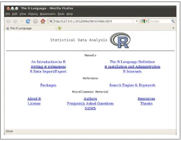
It is easy to browse this documentation via the help.start function, which opens a window on the top-level table of contents; see Figure 1-1.
Figure 1-1. Documentation table of contents
The two links in the Reference section are especially useful:
Packages
Click here to see a list of all the installed packages, both in the base packages and the additional installed packages. Click on a package name to see a list of its func-tions and datasets.
Search Engine & Keywords
Click here to access a simple search engine, which allows you to search the documentation by keyword or phrase. There is also a list of common keywords, organized by topic; click one to see the associated pages.
See Also
The local documentation is copied from the R Project website, which may have updated documents.
1.4 Searching the Web for Help
Problem
You want to search the Web for information and answers regarding R.
Solution
Inside R, use the RSiteSearch function to search by keyword or phrase:
> RSiteSearch("key phrase")
In your browser, try using these sites for searching:
http://rseek.org
This is a Google custom search that is focused on R-specific websites.
http://stackoverflow.com/
Stack Overflow is a searchable Q&A site oriented toward programming issues such as data structures, coding, and graphics.
http://stats.stackexchange.com/
The Statistical Analysis area on Stack Exchange is also a searchable Q&A site, but it is oriented more toward statistics than programming.
Discussion
The RSiteSearch function will open a browser window and direct it to the search engine on the R Project website (http://search.r-project.org/). There, you will see an initial search that you can refine. For example, this call would start a search for “canonical correlation”:
This is quite handy for doing quick Web searches without leaving R. However, the search scope is limited to R documentation and the mailing-list archives.
RSeek.org provides a wider search. Its virtue is that it harnesses the power of the Google search engine while focusing on sites relevant to R. That eliminates the extraneous results of a generic Google search. The beauty of RSeek.org is that it organizes the results in a useful way.
Figure 1-2 shows the results of visiting RSeek.org and searching for “canonical corre-lation”. The left side of the page shows general results for search R sites. The right side is a tabbed display that organizes the search results into several categories:
• Introductions • Task Views • Support Lists • Functions • Books • Blogs
• Related Tools
Figure 1-2. Search results from RSeek.org
If you click on the Introductions tab, for example, you’ll find tutorial material. The Task Views tab will show any Task View that mentions your search term. Likewise, clicking on Functions will show links to relevant R functions. This is a good way to zero in on search results.
Stack Overflow is a so-called Q&A site, which means that anyone can submit a question and experienced users will supply answers—often there are multiple answers to each question. Readers vote on the answers, so good answers tend to rise to the top. This creates a rich database of searchable Q&A dialogs. Stack Overflow is strongly problem oriented, and the topics lean toward the programming side of R.
Stack Overflow hosts questions for many programming languages; therefore, when entering a term into their search box, prefix it with “[r]” to focus the search on questions tagged for R. For example, searching for “[r] standard error” will select only the ques-tions tagged for R and will avoid Python and C++ quesques-tions.
Stack Exchange (not Overflow) has a Q&A area for Statistical Analysis. The area is more focused on statistics than programming, so use this site when seeking answers that are more concerned with statistics in general and less with R in particular.
See Also
If your search reveals a useful package, use the install.packages function to install it on your machine.
1.5 Reading Tabular Datafiles
Problem
You want to read a text file that contains a table of data.
Solution
Use the read.table function, which returns a data frame:
> dfrm <- read.table("filename.txt")
Discussion
Tabular datafiles are quite common. They are text files with a simple format: • Each line contains one record.
• Within each record, fields (items) are separated by a one-character delimiter, such as a space, tab, colon, or comma.
This format is more free-form than the fixed-width format because fields needn’t be aligned by position. Here is a datafile in tabular format, called statisticians.txt, using a space character between fields:
Fisher R.A. 1890 1962 Pearson Karl 1857 1936 Cox Gertrude 1900 1978 Yates Frank 1902 1994 Smith Kirstine 1878 1939
The read.table function is built to read this file. By default, it assumes the data fields are separated by white space (blanks or tabs):
> dfrm <- read.table("statisticians.txt")
> print(dfrm)
V1 V2 V3 V4 1 Fisher R.A. 1890 1962 2 Pearson Karl 1857 1936 3 Cox Gertrude 1900 1978 4 Yates Frank 1902 1994 5 Smith Kirstine 1878 1939
If your file uses a separator other than white space, specify it using the sep parameter. For example, if our file used a colon (:) as the field separator, we would read it this way:
> dfrm <- read.table("statisticians.txt", sep=":")
You can’t tell from the printed output, but read.table interpreted the first and last names as factors, not strings. We see that by checking the class of the resulting column:
> class(dfrm$V1)
[1] "factor"
To prevent read.table from interpreting character strings as factors, set the stringsAs Factors parameter to FALSE:
> dfrm <- read.table("statisticians.txt", stringsAsFactor=FALSE)
> class(dfrm$V1)
[1] "character"
Now the class of the first column is character, not factor.
If any field contains the string “NA”, then read.table assumes that the value is missing and converts it to NA. Your datafile might employ a different string to signal missing values; if it does, use the na.strings parameter. The SAS convention, for example, is that missing values are signaled by a single period (.). We can read such datafiles like this:
> dfrm <- read.table("filename.txt", na.strings=".")
I am a huge fan of self-describing data: datafiles which describe their own contents. (A computer scientist would say the file contains its own metadata.) The read.table func-tion has two features that support this characteristic. First, you can include a header line at the top of your file that gives names to the columns. The line contains one name
for every column, and it uses the same field separator as the data. Here is our datafile with a header line that names the columns:
lastname firstname born died Fisher R.A. 1890 1962 Pearson Karl 1857 1936 Cox Gertrude 1900 1978 Yates Frank 1902 1994 Smith Kirstine 1878 1939
Now we can tell read.table that our file contains a header line, and it will use the column names when it builds the data frame:
> dfrm <- read.table("statisticians.txt", header=TRUE, stringsAsFactor=FALSE)
> print(dfrm)
lastname firstname born died 1 Fisher R.A. 1890 1962 2 Pearson Karl 1857 1936 3 Cox Gertrude 1900 1978 4 Yates Frank 1902 1994 5 Smith Kirstine 1878 1939
The second feature of read.table is comment lines. Any line that begins with a pound sign (#) is ignored, so you can put comments on those lines:
# This is a datafile of famous statisticians. # Last edited on 1994-06-18
lastname firstname born died Fisher R.A. 1890 1962 Pearson Karl 1857 1936 Cox Gertrude 1900 1978 Yates Frank 1902 1994 Smith Kirstine 1878 1939
read.table has many parameters for controlling how it reads and interprets the input file. See the help page for details.
See Also
If your data items are separated by commas, see Recipe 1.6 for reading a CSV file.
1.6 Reading from CSV Files
Problem
You want to read data from a comma-separated values (CSV) file.
Solution
The read.csv function can read CSV files. If your CSV file has a header line, use this:
If your CSV file does not contain a header line, set the header option to FALSE:
> tbl <- read.csv("filename", header=FALSE)
Discussion
The CSV file format is popular because many programs can import and export data in that format. Such programs include R, Excel, other spreadsheet programs, many da-tabase managers, and most statistical packages. CSV is a flat file of tabular data, in which each line in the file is a row of data, and each row contains data items separated by commas. Here is a very simple CSV file with three rows and three columns (the first line is a header line that contains the column names, also separated by commas):
label,lbound,ubound low,0,0.674 mid,0.674,1.64 high,1.64,2.33
The read.csv function reads the data and creates a data frame, which is the usual R representation for tabular data. The function assumes that your file has a header line unless told otherwise:
> tbl <- read.csv("table-data.csv")
> tbl
label lbound ubound 1 low 0.000 0.674 2 mid 0.674 1.640 3 high 1.640 2.330
Observe that read.csv took the column names from the header line for the data frame. If the file did not contain a header, we would specify header=FALSE, and R would syn-thesize column names for us (V1, V2, and V3 in this case):
> tbl <- read.csv("table-data-with-no-header.csv", header=FALSE)
> tbl
V1 V2 V3 1 low 0.000 0.674 2 mid 0.674 1.640 3 high 1.640 2.330
A good feature of read.csv is that is automatically interprets nonnumeric data as a factor (categorical variable), which is often what you want since this is, after all, a statistical package, not Perl. The label variable in the tbl data frame just shown is actually a factor, not a character variable. You see that by inspecting the structure of tbl:
> str(tbl)
'data.frame': 3 obs. of 3 variables:
$ label : Factor w/ 3 levels "high","low","mid": 2 3 1 $ lbound: num 0 0.674 1.64
$ ubound: num 0.674 1.64 2.33
Sometimes, you really want your data interpreted as strings, not as factors. In that case, set the as.is parameter to TRUE; this indicates that R should not interpret nonnumeric data as a factor:
> tbl <- read.csv("table-data.csv", as.is=TRUE)
> str(tbl)
'data.frame': 3 obs. of 3 variables: $ label : chr "low" "mid" "high" $ lbound: num 0 0.674 1.64 $ ubound: num 0.674 1.64 2.33
Notice that the label variable now has character-string values and is no longer a factor. Another useful feature is that input lines starting with a pound sign (#) are ignored, which lets you embed comments in your datafile. Disable this feature by specifying comment.char="".
The read.csv function has many useful bells and whistles. These include the ability to skip leading lines in the input file, control the conversion of individual columns, fill out short rows, limit the number of lines, and control the quoting of strings. See the R help page for details.
See Also
See the R help page for read.table, which is the basis for read.csv. See the write.csv function for writing CSV files.
1.7 Creating a Vector
Problem
You want to create a vector.
Solution
Use the c(...) operator to construct a vector from given values.
Discussion
Vectors are a central component of R, not just another data structure. A vector can contain numbers, strings, or logical values, but not a mixture.
The c(...) operator can construct a vector from simple elements:
> c(1,1,2,3,5,8,13,21)
[1] 1 1 2 3 5 8 13 21 > c(1*pi, 2*pi, 3*pi, 4*pi)
[1] 3.141593 6.283185 9.424778 12.566371 > c("Everyone", "loves", "stats.")
[1] "Everyone" "loves" "stats." > c(TRUE,TRUE,FALSE,TRUE)
If the arguments to c(...) are themselves vectors, it flattens them and combines them into a single vector:
> v1 <- c(1,2,3)
> v2 <- c(4,5,6)
> c(v1,v2)
[1] 1 2 3 4 5 6
Vectors cannot contain a mix of data types, such as numbers and strings. If you create a vector from mixed elements, R will try to accommodate you by converting one of them:
> v1 <- c(1,2,3)
> v3 <- c("A","B","C")
> c(v1,v3)
[1] "1" "2" "3" "A" "B" "C"
Here, the user tried to create a vector from both numbers and strings. R converted all the numbers to strings before creating the vector, thereby making the data elements compatible.
Technically speaking, two data elements can coexist in a vector only if they have the same mode. The modes of 3.1415 and "foo" are numeric and character, respectively:
> mode(3.1415)
[1] "numeric" > mode("foo")
[1] "character"
Those modes are incompatible. To make a vector from them, R converts 3.1415 to character mode so it will be compatible with "foo":
> c(3.1415, "foo")
[1] "3.1415" "foo" > mode(c(3.1415, "foo"))
[1] "character"
c is a generic operator, which means that it works with many datatypes and not just vectors. However, it might not do exactly what you expect, so check its behavior before applying it to other datatypes and objects.
1.8 Computing Basic Statistics
Problem
You want to calculate basic statistics: mean, median, standard deviation, variance, correlation, or covariance.
Solution
Use one of these functions as appropriate, assuming that x and y are vectors:
• mean(x)
• median(x)
• sd(x)
• var(x)
• cor(x, y)
• cov(x, y)
Discussion
When I first opened the documentation for R, I began searching for material called something like “Procedures for Calculating Standard Deviation.” I figured that such an important topic would likely require a whole chapter.
It’s not that complicated.
Standard deviation and other basic statistics are calculated by simple functions. Ordi-narily, the function argument is a vector of numbers, and the function returns the calculated statistic:
> x <- c(0,1,1,2,3,5,8,13,21,34)
> mean(x)
[1] 8.8 > median(x)
[1] 4 > sd(x)
[1] 11.03328 > var(x)
[1] 121.7333
The sd function calculates the sample standard deviation, and var calculates the sample variance.
The cor and cov functions can calculate the correlation and covariance, respectively, between two vectors:
> x <- c(0,1,1,2,3,5,8,13,21,34)
> y <- log(x+1)
> cor(x,y)
[1] 0.9068053 > cov(x,y)
[1] 11.49988
All these functions are picky about values that are not available (NA). Even one NA value in the vector argument causes any of these functions to return NA, or even halt altogether with a cryptic error:
> x <- c(0,1,1,2,3,NA)
> mean(x)
[1] NA > sd(x)
It’s annoying when R is that cautious, but it is the right thing to do. You must think carefully about your situation. Does an NA in your data invalidate the statistic? If yes, then R is doing the right thing. If not, you can override this behavior by setting na.rm=TRUE, which tells R to ignore the NA values:
> x <- c(0,1,1,2,3,NA)
> mean(x, na.rm=TRUE)
[1] 1.4
> sd(x, na.rm=TRUE)
[1] 1.140175
A beautiful aspect of mean and sd is that they are smart about data frames. They un-derstand that each column of the data frame is a different variable, so they calculate their statistic for each column individually. This example calculates those basic statis-tics for a data frame with three columns:
> print(dframe)
small medium big 1 0.6739635 10.526448 99.83624 2 1.5524619 9.205156 100.70852 3 0.3250562 11.427756 99.73202 4 1.2143595 8.533180 98.53608 5 1.3107692 9.763317 100.74444 6 2.1739663 9.806662 98.58961 7 1.6187899 9.150245 100.46707 8 0.8872657 10.058465 99.88068 9 1.9170283 9.182330 100.46724 10 0.7767406 7.949692 100.49814 > mean(dframe)
small medium big 1.245040 9.560325 99.946003 > sd(dframe)
small medium big 0.5844025 0.9920281 0.8135498
Notice that mean and sd both return three values, one for each column defined by the data frame. (Technically, they return a three-element vector in which the names attribute is taken from the columns of the data frame.)
The var function understands data frames, too, but it behaves quite differently from mean and sd. It calculates the covariance between the columns of the data frame and returns the covariance matrix:
> var(dframe)
small medium big small 0.34152627 -0.21516416 -0.04005275 medium -0.21516416 0.98411974 -0.09253855 big -0.04005275 -0.09253855 0.66186326
Likewise, if x is either a data frame or a matrix, cor(x) returns the correlation matrix and cov(x) returns the covariance matrix:
> cor(dframe)
small medium big small 1.00000000 -0.3711367 -0.08424345 medium -0.37113670 1.0000000 -0.11466070 big -0.08424345 -0.1146607 1.00000000 > cov(dframe)
small medium big small 0.34152627 -0.21516416 -0.04005275 medium -0.21516416 0.98411974 -0.09253855 big -0.04005275 -0.09253855 0.66186326
Alas, the median function does not understand data frames. To calculate the medians of data frame columns, use the lapply function to apply the median function to each column separately.
See Also
See Recipe 1.12 for calculating the confidence interval of the mean. See Recipe 1.15 for testing the significance of a correlation.
1.9 Initializing a Data Frame from Column Data
Problem
Your data is organized by columns, and you want to assemble it into a data frame.
Solution
If your data is captured in several vectors and/or factors, use the data.frame function to assemble them into a data frame:
> dfrm <- data.frame(v1, v2, v3, f1, f2)
Use as.data.frame instead if your data is captured in a list that contains vectors and/ or factors:
> dfrm <- as.data.frame(list.of.vectors)
Discussion
A data frame is a collection of columns, each of which corresponds to an observed variable (in the statistical sense, not the programming sense). If your data is already organized into columns, then it’s easy to build a data frame.
> dfrm <- data.frame(pred1, pred2, pred3, resp)
> dfrm
pred1 pred2 pred3 resp 1 -2.7528917 -1.40784130 AM 12.57715 2 -0.3626909 0.31286963 AM 21.02418 3 -1.0416039 -0.69685664 PM 18.94694 4 1.2666820 -1.27511434 PM 18.98153 5 0.7806372 -0.27292745 AM 19.59455 6 -1.0832624 0.73383339 AM 20.71605 7 -2.0883305 0.96816822 PM 22.70062 8 -0.7063653 -0.84476203 PM 18.40691 9 -0.8394022 0.31530793 PM 21.00930 10 -0.4966884 -0.08030948 AM 19.31253
Notice that data.frame takes the column names from your program variables. You can override that default by supplying explicit column names:
> dfrm <- data.frame(p1=pred1, p2=pred2, p3=pred3, r=resp)
> dfrm
p1 p2 p3 r 1 -2.7528917 -1.40784130 AM 12.57715 2 -0.3626909 0.31286963 AM 21.02418 3 -1.0416039 -0.69685664 PM 18.94694 .
. (etc.)
.
Alternatively, your data may be organized into vectors, but those vectors are held in a list instead of individual program variables, like this:
> lst <- list(p1=pred1, p2=pred2, p3=pred3, r=resp)
No problem. Use the as.data.frame function to create a data frame from the list of vectors:
> as.data.frame(lst)
p1 p2 p3 r 1 -2.7528917 -1.40784130 AM 12.57715 2 -0.3626909 0.31286963 AM 21.02418 3 -1.0416039 -0.69685664 PM 18.94694 .
. (etc.)
.
1.10 Selecting Data Frame Columns by Position
Problem
You want to select columns from a data frame according to their position.
Solution
To select a single column, use this list operator:
dfrm[[n]]
Returns one column—specifically, the nth column of dfrm.
To select one or more columns and package them in a data frame, use the following sublist expressions:
dfrm[n]
Returns a data frame consisting solely of the nth column of dfrm. dfrm[c(n1, n2, ..., nk)]
Returns a data frame built from the columns in positions n1, n2, ..., nk of dfrm. You can use matrix-style subscripting to select one or more columns:
dfrm[, n]
Returns the nth column (assuming that n contains exactly one value). dfrm[, c(n1, n2, ..., nk)]
Returns a data frame built from the columns in positions n1, n2, ..., nk.
Note that the matrix-style subscripting can return two different data types (either col-umn or data frame) depending on whether you select one colcol-umn or multiple columns.
Discussion
There are a bewildering number of ways to select columns from a data frame. The choices can be confusing until you understand the logic behind the alternatives. As you read this explanation, notice how a slight change in syntax—a comma here, a double-bracket there — changes the meaning of the expression.
Let’s play with the population data for the 16 largest cities in the Chicago metropolitan area:
> suburbs
Use simple list notation to select exactly one column, such as the first column:
> suburbs[[1]]
[1] "Chicago" "Kenosha" "Aurora" "Elgin" [5] "Gary" "Joliet" "Naperville" "Arlington Heights" [9] "Bolingbrook" "Cicero" "Evanston" "Hammond" [13] "Palatine" "Schaumburg" "Skokie" "Waukegan"
The first column of suburbs is a vector, so that’s what suburbs[[1]] returns: a vector. If the first column were a factor, we’d get a factor.
The result differs when you use the single-bracket notation, as in suburbs[1] or suburbs[c(1,3)]. You still get the requested columns, but R wraps them in a data frame. This example returns the first column wrapped in a data frame:
> suburbs[1]
city 1 Chicago 2 Kenosha 3 Aurora 4 Elgin 5 Gary 6 Joliet 7 Naperville 8 Arlington Heights 9 Bolingbrook 10 Cicero 11 Evanston 12 Hammond 13 Palatine 14 Schaumburg 15 Skokie 16 Waukegan
The next example returns the first and third columns wrapped in a data frame:
> suburbs[c(1,3)]
city pop 1 Chicago 2853114 2 Kenosha 90352 3 Aurora 171782 4 Elgin 94487 5 Gary 102746 6 Joliet 106221 7 Naperville 147779 8 Arlington Heights 76031 9 Bolingbrook 70834 10 Cicero 72616 11 Evanston 74239 12 Hammond 83048 13 Palatine 67232 14 Schaumburg 75386 15 Skokie 63348 16 Waukegan 91452
A major source of confusion is that suburbs[[1]] and suburbs[1] look similar but pro-duce very different results:
suburbs[[1]]
This returns one column. suburbs[1]
This returns a data frame, and the data frame contains exactly one column. This is a special case of dfrm[c(n1,n2, ..., nk)]. We don’t need the c(...) construct
because there is only one n.
The point here is that “one column” is different from “a data frame that contains one column.” The first expression returns a column, so it’s a vector or a factor. The second expression returns a data frame, which is different.
R lets you use matrix notation to select columns, as shown in the Solution. But an odd quirk can bite you: you might get a column or you might get a data frame, depending which many subscripts you use. In the simple case of one index you get a column, like this:
> suburbs[,1]
[1] "Chicago" "Kenosha" "Aurora" "Elgin" [5] "Gary" "Joliet" "Naperville" "Arlington Heights" [9] "Bolingbrook" "Cicero" "Evanston" "Hammond" [13] "Palatine" "Schaumburg" "Skokie" "Waukegan"
But using the same matrix-style syntax with multiple indexes returns a data frame:
> suburbs[,c(1,4)]
city pop 1 Chicago 2853114 2 Kenosha 90352 3 Aurora 171782 4 Elgin 94487 5 Gary 102746 6 Joliet 106221 7 Naperville 147779 8 Arlington Heights 76031 9 Bolingbrook 70834 10 Cicero 72616 11 Evanston 74239 12 Hammond 83048 13 Palatine 67232 14 Schaumburg 75386 15 Skokie 63348 16 Waukegan 91452
This creates a problem. Suppose you see this expression in some old R script:
dfrm[,vec]
To avoid this problem, you can include drop=FALSE in the subscripts; this forces R to return a data frame:
dfrm[,vec,drop=FALSE]
Now there is no ambiguity about the returned data structure. It’s a data frame. When all is said and done, using matrix notation to select columns from data frames is not the best procedure. I recommend that you instead use the list operators described previously. They just seem clearer.
1.11 Selecting Data Frame Columns by Name
Problem
You want to select columns from a data frame according to their name.
Solution
To select a single column, use one of these list expressions:
dfrm[["name"]]
Returns one column, the column called name. dfrm$name
Returns the same, but presented in different syntax.
To select one or more columns and package them in a data frame, use these list expressions:
dfrm["name"]
Selects one column and packages it inside a data frame object. dfrm[c("name1", "name2", ..., "namek")]
Selects several columns and packages them in a data frame. You can use matrix-style subscripting to select one or more columns:
dfrm[, "name"]
Returns the named column.
dfrm[, c("name1", "name2", ..., "namek")]
Selects several columns and packages them in a data frame.
Once again, the matrix-style subscripting can return two different data types (column or data frame) depending on whether you select one column or multiple columns.
Discussion
All columns in a data frame must have names. If you know the name, it’s usually more convenient and readable to select by name, rather than by position.
The solutions just described are similar to those for Recipe 1.10, where we selected columns by position. The only difference is that here we use column names instead of column numbers. All the observations made in Recipe 1.10 apply here:
• dfrm[["name"]] returns one column, not a data frame.
• dfrm[c("name1", "name2", ..., "namek")] returns a data frame, not a column. • dfrm["name"] is a special case of the previous expression and so returns a data frame,
not a column.
• The matrix-style subscripting can return either a column or a data frame, so be careful how many names you supply. See Recipe 1.10 for a discussion of this “gotcha” and using drop=FALSE.
There is one new addition:
dfrm$name
This is identical in effect to dfrm[["name"]], but it’s easier to type and to read.
See Also
See Recipe 1.10 to understand more about selecting columns.
1.12 Forming a Confidence Interval for a Mean
Problem
You have a sample from a population. Given that sample, you want to determine a confidence interval for the population’s mean.
Solution
Apply the t.test function to your sample x:
> t.test(x)
The output includes a confidence interval at the 95% confidence level. To see intervals at other levels, use the conf.level argument.
If your sample size n is small, the underlying population must be normally distributed for there to be a meaningful confidence interval. A good rule of thumb is that “small” means n < 30.
Discussion
> x <- rnorm(50, mean=100, sd=15)
> t.test(x)
One Sample t-test data: x
t = 59.2578, df = 49, p-value < 2.2e-16
alternative hypothesis: true mean is not equal to 0 95 percent confidence interval:
97.16167 103.98297 sample estimates: mean of x 100.5723
In this example, the confidence interval is approximately 97.16 < μ < 103.98, which is
sometimes written simply as (97.16, 103.98).
We can raise the confidence level to 99% by setting conf.level=0.99:
> t.test(x, conf.level=0.99)
One Sample t-test data: x
t = 59.2578, df = 49, p-value < 2.2e-16
alternative hypothesis: true mean is not equal to 0 99 percent confidence interval:
96.0239 105.1207 sample estimates: mean of x 100.5723
That change widens the confidence interval to 96.02 < μ < 105.12.
1.13 Forming a Confidence Interval for a Proportion
Problem
You have a sample of values from a population consisting of successes and failures. Based on the sample data, you want to form a confidence interval for the population’s proportion of successes.
Solution
Use the prop.test function. Suppose the sample size is n and the sample contains x successes:
> prop.test(n, x)
The function output includes the confidence interval for p.
Discussion
I subscribe to a stock market newsletter that is well written for the most part, but includes a section purporting to identify stocks that are likely to rise. It does this by looking for a certain pattern in the stock price. It recently reported, for example, that a certain stock was following the pattern. It also reported that the stock rose six times after the last nine times that pattern occurred. The writers concluded that the proba-bility of the stock rising again was therefore 6/9 or 66.7%.
Using prop.test, we can obtain the confidence interval for the true proportion of times the stock rises after the pattern. Here, the number of observations is n = 9 and the number of successes is x = 6. The output shows a confidence interval of (0.309, 0.910) at the 95% confidence level:
> prop.test(6, 9)
1-sample proportions test with continuity correction data: 6 out of 9, null probability 0.5
X-squared = 0.4444, df = 1, p-value = 0.505 alternative hypothesis: true p is not equal to 0.5 95 percent confidence interval:
0.3091761 0.9095817 sample estimates: p 0.6666667
The writers are pretty foolish to say the probability of rising is 66.7%. They could be leading their readers into a very bad bet.
By default, prop.test calculates a confidence interval at the 95% confidence level. Use the conf.level argument for other confidence levels, like this:
> prop.test(n, x, p, conf.level=0.99) # 99% confidence level
1.14 Comparing the Means of Two Samples
Problem
You have one sample each from two populations. You want to know if the two popu-lations could have the same mean.
Solution
Perform a t test by calling the t.test function:
> t.test(x, y)
By default, t.test assumes that your data is not paired. If the observations are paired (i.e., if each xi is paired with the corresponding yi), then specify paired=TRUE:
In either case, t.test will compute a p-value. Conventionally, if p < 0.05, the means are likely different, whereas p > 0.05 provides no such evidence:
• If either sample size is small, the populations must be normally distributed. Here, “small” means fewer than 20 data points.
• If the two populations have the same variance, specify var.equal=TRUE to obtain a less conservative test.
Discussion
I often use the t test to get a quick sense of the difference between two population means. It requires that the samples be large enough—both samples have 20 or more observations—or that the underlying populations be normally distributed. I don’t take the “normally distributed” part too literally. Being bell-shaped should be good enough. A key distinction here is whether your data contains paired observations, since the answer may cause your results to differ. Suppose we want to know if coffee in the morning improves scores on SAT tests. We could run the experiment two ways:
• Randomly select one group of people. Give them the SAT test twice, once with morning coffee and once without morning coffee. For each person, we will have two SAT scores. These are paired observations.
• Randomly select two groups of people. One group has a cup of morning coffee and takes the SAT test. The other group just takes the test. We have a score for each person, but the scores are not paired in any way.
Statistically, these experiments are quite different. In experiment 1, there are two observations for each person (caffeinated and decaf) and they are not statistically in-dependent. In experiment 2, the data is inin-dependent.
If you have paired observations (experiment 1) and erroneously analyze them as un-paired observations (experiment 2), then you could get this result with a p-value of 0.9867:
> t.test(x,y)
Welch Two Sample t-test data: x and y
t = -0.0166, df = 198, p-value = 0.9867
alternative hypothesis: true difference in means is not equal to 0 95 percent confidence interval:
-30.56737 30.05605 sample estimates: mean of x mean of y 501.2008 501.4565
The large p-value forces you to conclude that there is no difference between the groups. Contrast that result with the one from analyzing the same data, but correctly identifying it as paired:
> t.test(x, y, paired=TRUE)
Paired t-test data: x and y
t = -2.3636, df = 99, p-value = 0.02005
alternative hypothesis: true difference in means is not equal to 0 95 percent confidence interval:
-0.4702824 -0.0410375 sample estimates: mean of the differences -0.2556599
The p-value plummets to 0.02005, and we reach exactly the opposite conclusion.
See Also
If the populations are not normally distributed (bell-shaped) and either sample is small, the t test is inappropriate. In that case, consider using the Wilcoxon-Mann-Whitney test, which is implemented by the wilcox.test function.
1.15 Testing a Correlation for Significance
Problem
You calculated the correlation between two variables, but you don’t know if the cor-relation is statistically significant.
Solution
The cor.test function can calculate both the p-value and the confidence interval of the correlation. If the variables came from normally distributed populations, use the default measure of correlation, known as the Pearson method:
> cor.test(x, y)
For nonnormal populations, use the Spearman method instead:
> cor.test(x, y, method="Spearman")
The function returns several values, including the p-value from the test of significance. Conventionally, p < 0.05 indicates that the correlation is likely significant, whereas p
Discussion
In my experience, people often fail to check a correlation for significance. In fact, many people are unaware that a correlation can be insignificant. They jam their data into a computer, calculate the correlation, and blindly believe the result. However, they should ask themselves: Was there enough data? Is the magnitude of the correlation large enough? Fortunately, the cor.test function answers those questions.
Suppose we have two vectors, x and y, with values from normal populations. We might be very pleased that their correlation is greater than 0.83:
> cor(x, y)
[1] 0.8352458
But that is naïve. If we run cor.test, it reports a relatively large p-value of 0.1648:
> cor.test(x, y)
Pearson's product-moment correlation data: x and y
t = 2.1481, df = 2, p-value = 0.1648
alternative hypothesis: true correlation is not equal to 0 95 percent confidence interval:
-0.6379590 0.9964437 sample estimates: cor 0.8352458
The p-value is above the conventional threshold of 0.05, so we conclude that the cor-relation is unlikely to be significant.
You can also check the correlation by using the confidence interval. In this example, the confidence interval is (−0.638, 0.996). The interval contains zero, so it is possible that the correlation is zero, in which case there would be no correlation. Again, you could not be confident that the reported correlation is significant.
The cor.test output also includes the point estimate reported by cor (at the bottom, labeled “sample estimates”), saving you the additional step of running cor.
By default, cor.test calculates the Pearson correlation, which assumes that the under-lying populations are normally distributed. The Spearman method makes no such as-sumption because it is nonparametric. Use method="Spearman" when working with nonnormal data.
See Also
See Recipe 1.8 for computing correlations and other basic statistics.
1.16 Creating a Scatter Plot
Problem
You have paired observations: (x1, y1), (x2, y2), ..., (xn, yn). You want to create a scatter plot of the pairs.
Solution
If your data is held in two parallel vectors, x and y, use them as arguments of plot:
> plot(x, y)
If your data is held in a (two-column) data frame, plot the data frame:
> plot(dfrm)
Discussion
A scatter plot is usually my first attack on a new dataset. It’s a quick way to see the relationship, if any, between x and y. Creating the scatter plot is easy:
> plot(x, y)
The plot function does not return anything. Rather, its purpose is to draw a plot of the (x, y) pairs in the graphics window.
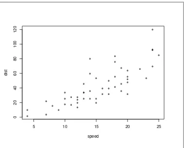
Life is even easier if your data is captured in a two-column data frame. If you plot a two-column data frame, the function assumes you want a scatter plot created from those two columns. The scatter plot shown in Figure 1-3 was created by one call to plot:
> plot(cars)
The cars dataset contains two columns: speed and dist. The first column is speed, so that becomes the x-axis, and dist becomes the y-axis.
If your data frame contains more than two columns, you will get multiple scatter plots, which might or might not be useful.
To get a scatter plot, your data must be numeric. Recall that plot is a polymorphic function, so, if the arguments are nonnumeric, it will create some other type of plot. See Recipe 1.18, for example, which creates box plots from factors.
See Also
1.17 Creating a Bar Chart
Problem
You want to create a bar chart.
Solution
Use the barplot function. The first argument is a vector of bar heights:
> barplot(c(height1, height2, height3))
Discussion
The barplot function produces a simple bar chart. It assumes that the heights of your bars are conveniently stored in a vector. That is not always the case, however. Often, you have a vector of numeric data and a parallel factor that groups the data, and you want to produce a bar chart of the group means or the group totals. For example, the airquality dataset contains a numeric Temp column and a Month column. We can create
● ● ● ● ● ● ● ● ● ● ● ● ● ● ● ● ● ● ● ● ● ● ● ● ● ● ● ● ● ● ● ● ● ● ● ● ● ● ● ● ● ● ● ● ● ● ● ● ● ●
5 10 15 20 25
0 20 40 60 80 100 120 speed dist
Figure 1-3. Scatter plot
a bar chart of the mean temperature by month in two steps. First, we compute the means:
> heights <- tapply(airquality$Temp, airquality$Month, mean)
That gives the heights of the bars, from which we create the bar chart:
> barplot(heights)
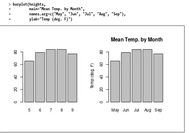
The result is shown in the lefthand panel of Figure 1-4. The result is pretty bland, as you can see, so it’s common to add some simple adornments: a title, labels for the bars, and a label for the y-axis:
> barplot(heights,
+ main="Mean Temp. by Month",
+ names.arg=c("May", "Jun", "Jul", "Aug", "Sep"),
+ ylab="Temp (deg. F)")
5 6 7 8 9
0
20
40
60
80
May Jun Jul Aug Sep
Mean Temp. by Month
T
emp (deg. F)
0
20
40
60
80
Figure 1-4. Bar charts, plain (left) and adorned (right)
The righthand panel of Figure 1-4 shows the improved bar chart.
See Also
The barchart function in the lattice package is another way to produce a bar chart.
1.18 Creating a Box Plot
Problem
Solution
Use boxplot(x), where x is a vector of numeric values.
Discussion
A box plot provides a quick and easy visual summary of a dataset. Figure 1-5 shows a typical box plot:
• The thick line in the middle is the median.
• The box surrounding the median identifies the first and third quartiles; the bottom of the box is Q1, and the top is Q3.
• The “whiskers” above and below the box show the range of the data, excluding outliers.
• The circles identify outliers. By default, an outlier is defined as any value that is farther than 1.5 × IQR away from the box. (IQR is the interquartile range, or Q3 − Q1.) In this example, there are three outliers.
● ● ●
0
1
2
3
4
Figure 1-5. Your typical box plot
1.19 Creating a Histogram
Problem
You want to create a histogram of your data.
Solution
Use hist(x), where x is a vector of numeric values.
Discussion
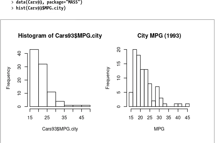
The lefthand panel of Figure 1-6 shows a histogram of the MPG.city column taken from the Cars93 dataset, created like this:
> data(Cars93, package="MASS")
> hist(Cars93$MPG.city)
Histogram of Cars93$MPG.city
Cars93$MPG.city
Frequency
15 25 35 45
0
10
20
30
40
City MPG (1993)
MPG
Frequency
15 20 25 30 35 40 45
0
5
10
15
20
Figure 1-6. Histograms
The hist function must decide how many cells (bins) to create for binning the data. In this example, the default algorithm chose seven bins. That creates too few bars for my taste, because the shape of the distribution remains hidden. So, I would include a sec-ond argument for hist—namely, the suggested number of bins:
> hist(Cars93$MPG.city, 20)
The righthand panel of Figure 1-6 shows a histogram for the same data, but with more bins and with replacements for the default title and x-axis label. It was created like this:
> hist(Cars93$MPG.city, 20, main="City MPG (1993)", xlab="MPG")
See Also
The histogram function of the lattice package is an alternative to hist.
1.20 Performing Simple Linear Regression
Problem
You have two vectors, x and y, that hold paired observations: (x1, y1), (x2, y2), ..., (xn, yn). You believe there is a linear relationship between x and y, and you want to create a regression model of the relationship.
Solution
The lm function performs a linear regression and reports the coefficients:
> lm(y ~ x)
Call:
lm(formula = y ~ x) Coefficients:
(Intercept) x 17.72 3.25
Discussion
Simple linear regression involves two variables: a predictor variable, often called x; and a response variable, often called y. The regression uses the ordinary least-squares (OLS) algorithm to fit the linear model:
yi = β0 + β1xi + εi
where β0 and β1 are the regression coefficients and εi represents the error terms. The lm function can perform linear regression. The main argument is a model formu-la, such as y ~ x. The formula has the response variable on the left of the tilde character (~) and the predictor variable on the right. The function estimates the regression coef-ficients, β0 and β1, and reports them as the intercept and the coefficient of x,
respectively:
Coefficients:
(Intercept) x 17.72 3.25
In this case, the regression equation is:
yi = 17.72 + 3.25xi + εi
It is quite common for data to be captured inside a data frame, in which case you want to perform a regression between two data frame columns. Here, x and y are columns of a data frame dfrm:
> dfrm
x y 1 0.04781401 5.406651 2 1.90857986 19.941568 3 2.79987246 23.922613 4 4.46755305 32.432904 5 3.76490363 44.259268 6 5.92364632 61.151480 7 8.04611587 26.305505 8 7.11097986 43.606087 9 9.73645966 58.262112 10 9.19324543 57.631029 .
. (etc.)
.
The lm function lets you specify a data frame by using the data parameter. If you do, the function will take the variables from the data frame and not from your workspace:
> lm(y ~ x, data=dfrm) # Take x and y from dfrm Call:
lm(formula = y ~ x, data = dfrm) Coefficients:
(Intercept) x 17.72 3.25
1.21 Performing Multiple Linear Regression
Problem
You have several predictor variables (e.g., u, v, and w) and a response variable (y). You believe there is a linear relationship between the predictors and the response, and you want to perform a linear regression on the data.
Solution
Use the lm function. Specify the multiple predictors on the righthand side of the for-mula, separated by plus signs (+):
Discussion
Multiple linear regression is the obvious generalization of simple linear regression. It allows multiple predictor variables instead of one predictor variable and still uses OLS to compute the coefficients of a linear equation. The three-variable regression just shown corresponds to this linear model:
yi = β0 + β1ui + β2vi + β3wi + εi
R uses the lm function for both simple and multiple linear regression. You simply add more variables to the righthand side of the model formula. The output then shows the coefficients of the fitted model:
> lm(y ~ u + v + w)
Call:
lm(formula = y ~ u + v + w) Coefficients:
(Intercept) u v w 1.4222 1.0359 0.9217 0.7261
The data parameter of lm is especially valuable when the number of variables increases, since it’s much easier to keep your data in one data frame than in separate variables. Suppose your data is captured in a data frame, such as the dfrm variable shown here:
> dfrm
y u v w 1 6.584519 0.79939065 2.7971413 4.366557 2 6.425215 -2.31338537 2.7836201 4.515084 3 7.830578 1.71736899 2.7570401 3.865557 4 2.757777 1.27652888 0.4191765 2.547935 5 5.794566 0.39643488 2.3785468 3.265971 6 7.314611 1.82247760 1.8291302 4.518522 7 2.533638 -1.34186107 2.3472593 2.570884 8 8.696910 0.75946803 3.4028180 4.442560 9 6.304464 0.92000133 2.0654513 2.835248 10 8.095094 1.02341093 2.6729252 3.868573 .
. (etc.)
.
When we supply dfrm to the data parameter of lm, R looks for the regression variables in the columns of the data frame:
> lm(y ~ u + v + w, data=dfrm) Call:
lm(formula = y ~ u + v + w, data = dfrm) Coefficients:
(Intercept) u v w 1.4222 1.0359 0.9217 0.7261
See Also
See Recipe 1.20 for simple linear regression.
1.22 Getting Regression Statistics
Problem
You want the critical statistics and information regarding