El e c t ro n ic
Jo ur
n a l o
f P
r o
b a b il i t y
Vol. 15 (2010), Paper no. 59, pages 1825–1862. Journal URL
http://www.math.washington.edu/~ejpecp/
On clusters of high extremes of Gaussian stationary
processes with
ǫ-separation
Jürg Hüsler
∗Dept. of math. Statistics University of Bern
Anna Ladneva and Vladimir Piterbarg
†Faculty of Mechanics and Mathematics Moscow Lomonosov State University
Abstract
The clustering of extremes values of a stationary Gaussian processX(t),t∈[0,T]is considered, where at least two time points of extreme values above a high threshold are separated by at least a small positive value ǫ. Under certain assumptions on the correlation function of the process, the asymptotic behavior of the probability of such a pattern of clusters of exceedances is derived exactly where the level to be exceeded by the extreme values, tends to∞. The excursion behaviour of the paths in such an event is almost deterministic and does not depend on the high levelu. We discuss the pattern and the asymptotic probabilities of such clusters of exceedances.
Key words:Gaussian process, extreme values, clusters, separated clusters, asymptotic behavior, correlation function.
AMS 2000 Subject Classification:Primary 60G70; 60G15; 60G10.
Submitted to EJP on May 12, 2010, final version accepted October 18, 2010.
∗Supported in parts by Swiss National Science Foundation. E-mail: [email protected]
†Supported in parts by RFFI Grant 07-01-00077 of Russian Federation, grant DFG 436 RUS 113/722, and Swiss
1
Introduction and main results
LetX(t), t∈R, be a zero mean stationary, a.s. continuous Gaussian process with unit variance and covariance function r(t). We study probabilities of high extremes of the process. It is known that given a high extreme occurs in a bounded interval[0,T], say, then the excursion set
E(u,T):={t∈[0,T]: X(t)>u}
is non-empty, but typically very short. To prove this, one has to investigate mainly the conditional expectation of X(t)given X(0) =u1, where u1 is close to u, i.e. E(X(t)|X(0) =u1) =u1r(t)and to notice that the conditional covariance function does not depend onu1. It is necessary to assume
that r(t)is sufficiently regular at zero and r(t)< r(0)for all t >0. Applying then usual Gaussian asymptotical techniques, one can determine the corresponding asymptotically exact results. See for details, Berman[3], Piterbarg[8]. Notice also that high values of a Gaussian process with excursions above a high level occur rarely, and for non differentiable paths there are infinitely many crossings of the high level in a short interval, which tends to 0 as the levelu→ ∞. Hence, they are not separated by a fixedǫ, so that to use Gaussian processes modeling for ”physically significant” extremes one should consider larger excursions. In other words, considering a lower high levelu, one may observe longer excursions. To gain more insight in the extremal behavior of Gaussian processes, a natural step in studying high excursions is the consideration of the excursion sets, containing two points separated by some fixedǫ >0. Thus let us define the setEǫ(u,T)by
Eǫ(u,T):={∃s,t∈[0,T]:X(s)>u,t≥s+ǫ,X(t)>u}.
We show here that for particular correlation functions r(t), the trajectories spend a non-vanishing time aboveugiven the two separated excursionsX(s)>uandX(t)>u, asu→ ∞.
In order to study a limit structure of such excursion sets, we introduce the collection of eventsS
S :=
{inf
v∈AX(v)≥u, supv∈BX(v)≤u},A,B∈ C
(Astands forabove, B forbelow), whereC denotes the collection of all closed subsets ofR. Denote
by{Ts, s∈R}the group of shifts along trajectories of the processX(t). The family of probabilities
Pǫ,u,T(S):=P(∃s,t∈[0,T], t≥s+ǫ: X(s)>u,X(t)>u,TsS), S∈ S,
describes the structure of the extremes containing two excursions points separated by at leastǫ. We study the asymptotic behavior of this probability when u → ∞, which depends on the particular behavior ofr(t).
We describe the possible setsAwith excursions aboveugiven two exceedances which are at least ǫ separated. Furthermore, we can also describe in this case the sets B on which the trajectories are typically below u. Thus we study here the asymptotic behavior of the probability of "physi-cal extremes", that is, the probability of existence of excursions above a high level with physi"physi-cally significant duration.
Related problems were considered in Piterbarg and Stamatovic[9], where the asymptotic behaviour of the logarithm of the probability was derived for general Gaussian processes, where the setsAand
the probability of joint high values of two Gaussian processes. Clustering of extremes in time series data is a subject of modeling, e.g. in mathematical finances, meteorological studies, or reliability theory. The paper by Leadbetter et al.[5]presents some theoretical background for studying clusters of time series.
Our results depend on the behavior of the correlation function r(t)of the Gaussian process X(t). We introduce the following assumptions.
C1 For someα∈(0, 2),
r(t) =1− |t|α+o(|t|α) as t→0,
r(t)<1 for all t>0.
The behavior of the clustering depends on the maximal value of r(t) with
t∈[ǫ,T]. Thus we restrictr(t)in[ǫ,T]by the following conditions.
C2 In the interval[ǫ,T]there exists only one pointtmof maximumr(t)being an interior point of the interval: tm=arg max[ǫ,T]r(t)∈(ǫ,T), wherer(t)is twice continuously differentiable in
a neighborhood oftm withr′′(tm)<0.
The following condition deals with the case tm = ǫ, which seems somewhat more common since
r(t)decreases in a right neighborhood of zero. Unfortunately considerations in this case are more complicated.
C3 Assume that r(t) is continuously differentiable in a neighborhood of the point ǫ < T, with
r′(ǫ)<0, andr(ǫ)>r(t)for allt∈(ǫ,T], hencetm=ǫ.
Denote byBα(t), t∈R, the fractional Brownian motion with the Hurst parameterα/2∈(0, 1), that
is a Gaussian process with a.s. continuous trajectories, and with Bα(0) =0 a.s., EBα(t)≡ 0, and
E(Bα(t)−Bα(s))2=|t−s|α. For any setI⊂Rand a numberc≥0, we denote
Hα,c(I) =Eexp
sup t∈I
p
2Bα(t)− |t|α−c t
.
It is known, from Pickands[7]and Piterbarg[8], that there exist positive and finite limits
Hα:= lim λ→∞
1
λHα,0([0,λ]) (Pickands’ constant) (1)
Hα,c:= lim
λ→∞Hα,c([0,λ]), forc>0. (2)
Now consider the asymptotic expression for the joint exceedances of the leveluby the two r.v.’sX(0)
andX(t), i.e. for anyt>0,
P(X(0)>u,X(t)>u) = Ψ2(u,r(t))(1+o(1))
asu→ ∞, where
Ψ2(u,r) = (1+r)
3/2
2πu2p1−r exp
− u
2
1+r
The shape of excursion sets depends on the behavior of the conditional mean m(v): m(v) = E(X(v)| X(0) =X(tm) =1)which is
m(v) = r(v) +r(tm−v)
1+r(tm) .
Let
A0:={v:m(v)>1} and B0:={v:m(v)<1}.
We split the collection of eventsS into two sub-collectionsS0 andS1. The first sub-collectionS0
consists of the events generated by all closed subsets A⊂ A0, and all closed subsets B ⊂ B0, and the second sub-collectionS1 is its complement,S1 =S \ S0, generated by all closedA,B, having non-empty intersections withB0 or A0, respectively, A∩B0 6=;or B∩A0 6=;. Let us single out an
eventS∈ S withA=B=;, it equalsΩwith probability one, since trajectories ofX are continuous and we can simply write in this caseS= Ω. Clearly, we haveΩ∈ S0.
The probability
P(u;ǫ,T):=Pu;ǫ,T(Ω) =P(∃s,t∈[0,T]: t≥s+ǫ,X(s)≥u,X(t)≥u)
plays the crucial role in the study of asymptotic behavior of the set of exceedances. It turns out that the eventsS fromS0 give no contribution in the asymptotic behavior of the probability Pu;ǫ,T(S). Conversely, consideringS ∈ S1makes the probability exponentially smaller. Our main results show
the equivalence
Pǫ,u,T(S)∼P(u;ǫ,T), S∈ S0, (3) moreover, we give asymptotic expressions for P(u;ǫ,T) and exponential bounds for Pǫ,u,T(S),S ∈ S1. Note, this means that for anyA⊂A0we havePǫ,u,T(A) =P{∃t: mins∈A+tX(s)>u} ∼P(u;ǫ,T) asu→ ∞.
Theorem 1. Let X(t), t ∈R, be a Gaussian centered stationary process with a.s. continuous
trajecto-ries. Assume that the correlation function r(t)satisfiesC1and C2. Then we have the following.
(i) For any S∈ S0,
Pǫ,u,T(S) =
(T−tm)
p
2πHα2u−1+4/α
p
−r′′(tm)(1+r(tm))−1+4/α
Ψ2(u,r(tm))(1+o(1))
as u→ ∞.
(ii) For any S∈ S1there exists aδ >0with
Pǫ,u,T(S) =o
e−δu2Ψ2(u,r(tm))
as u→ ∞.
For the next results we need the following constanth. It is defined as
h=lim inf
λ→∞ lim infµ→∞
h1(λ,µ)
µ =lim supλ→∞
lim sup
µ→∞
h1(λ,µ)
withh1(λ,µ) =
=
Z Z
R2
ex+yP [
D
{p2B1(s)−(1+r′(ǫ))s> x,p2eB1(t)−(1−r′(ǫ))t> y}d x d y<∞,
where D={(s,t): 0≤s≤µ/(1+r(ǫ))2, 0≤ t−s≤λ/(1+r(ǫ))2} andB1(t)and Be1(t)denote independent copies of the standard Brownian motion.
Theorem 2. Let X(t), t ∈R, be a Gaussian centered stationary process with a.s. continuous
trajecto-ries. Assume that the correlation function r(t)satisfiesC1andC3. Then the following assertions take place.
1.If S∈ S0,then we have: (i)forα >1,
Pu;ǫ,T(S) = (T−ǫ)|r ′(ǫ)|
(1+r(ǫ))2 u
2Ψ
2(u,r(ǫ))(1+o(1)).
(ii)Forα=1,
Pu;ǫ,T(S) = (T−ǫ)hu2Ψ2(u,r(ǫ))(1+o(1)).
(iii)Forα <1,
Pu;ǫ,T(S) =
(T−ǫ)Hα2u−2+4/α
|r′(ǫ)|(1+r(ǫ))−2+4/αΨ2(u,r(ǫ))(1+o(1)).
2.If S∈ S1, then there existsδ >0such that Pu;ǫ,T(S) =o
e−δu2Ψ2(u,r(ǫ))as u→ ∞.
Remark 1:Notice that the relation (3) follows by letting in both TheoremsS= Ω∈ S0.
Remark 2: We do not consider the case of differentiable processes,α=2, because such
considera-tions require quite different arguments. This case will be considered in a separate publication. In addition, we do not care about the pointst such thatr(t) =−1, because they can be deleted in the derivations, as can be noted in the proofs.
The necessary lemmas for the proof of the two results are treated in Section 3, in Section 4 follows the proof of the main results. In the next section we first discuss some examples to indicate the pattern of exceedances depending on the given correlation function.
2
Examples
A general property in case of C3: If r(v) is above the straight line traced between (0, 1) and
(ǫ,r(ǫ)), then m(v) > 1 for all v ∈ (0,ǫ). Indeed, in this case r(v) > 1−(1−r(ǫ))v/ǫ and
r(ǫ−v)>1−(1−r(ǫ))(ǫ−v)/ǫ. Summing we get r(v) +r(ǫ−v)>1+r(ǫ). In particular, this holds ifr(t)is strictly concave on[0,ǫ]. It means that in this caseA0 contains(0,ǫ).
Example 1: Consider the correlation function
being the product of two correlation functions. It has countable many local maxima with decreasing heights. The first three local maxima after 0 aret(1)m ≈2.055, t(2)m ≈4.115,t(3)m ≈6.175. Fork≥1, denote bysk, the maximal root of the equation r(s) =r(t(mk))withs<t
(k)
m ,s1≈0.294,s2≈ 2.544,
s3≈4.734, (see Figure 1). Let T be larger than the consideredt(mk), withkfixed.
Ifǫhas been chosen betweens1andt(1)m , thentm=t(1)m andA0=;. It means that a typical trajectory with two such separated exceedances crosses (perhaps infinitely many times) a high levelu, but only in two very short (vanishing asu→ ∞) intervals concentrated around two points separated bytm, approximately.
If ǫ is larger, ǫ ∈ (s2,t(2)m ), then tm = t(2)m , A0 is non-empty, A0 ≈ (1.82, 2.29) (see Fig. 2). That is, given two exceedances of a high level u separated by at least such an ǫ, say, X(t1) > u and
X(t2) > u, t2−t1 ≥ ǫ, one observes between the exceedances an interval (not tending to 0) on
which the trajectory is aboveu. This interval is approximately congruent toA0. Note thatt2is rather close tot1+t(2)m for largeu.
Furthermore, ifǫ∈(s3,t(3)m ), thentm=t(3)m andA0≈(1.80, 2.31)∪(3.86, 4.37)(see Fig. 2), implying
in the case of two exceedances separated by at leastǫthat one observes two intervals on which the corresponding trajectory is entirely aboveu.
1 2 3 4 5 6 7 8 9 10
0.2 0.4 0.6 0.8
1.0 Correlation function r(t)
t
t(1)m t(2)m t(3)m t(4)m
s1 s2 s3 s4
Figure 1: Correlation functionr(t)of the example with the local maximat(mk)and the corresponding valuessk.
Theorem 2 can be used for the other cases ofǫ. The correlation functionr(t)is strictly concave on
(0,s1). For any positiveǫ∈(0,s1]we have alsor(t)<r(ǫ)for allt> ǫ. Thus, for suchǫ, Condition
C3 holds and thus Theorem 2 can be applied withA0 = (0,ǫ). It is easy to verify that m(v) <1 outside of[0,ǫ].
If ǫ ∈ (tm(1),s2), one can derive that A0 consists of two separated intervals (0,κ)∪(ǫ−κ,ǫ). For
example, forǫ=2.3, we get κ≈0.22. The ConditionsC1 andC3 are fulfilled, so the assertion (i) of Theorem 2 holds, but not the assertion of Corollary 3.
1 2 3 4 5 6 0.3
0.5 0.7 0.9 1.1
Conditional mean function m(v) for the third local maximat(3)m
v
A0 A0 t(3)m
1 2 3 4 5 6
0.3 0.5 0.7 0.9 1.1
Conditional mean function m(v) for the third local maximat(3)m
v
A0 A0 t(3)m
Figure 2: Conditional mean functionm(v)for the second and third local maxima t(mi),i=2, 3, with the corresponding setsA0
uwithǫ-separation.
Example 2: Consider the correlation function r(t) = exp(−|t|α), α ∈(0, 2). For any ǫ > 0, the
pointǫis the maximal point ofr(t)on[ǫ,∞). This is the situation ofC3.
If α≤ 1, then r(t)is convex and it can be determined that m(v)< 1 for all v 6∈ {0,ǫ}. We have
m(v) =1 forv∈ {0,ǫ}. ThusA0 is empty.
Ifα >1, r(t)is concave in a neighborhood of zero, as long as 0< t <[(α−1)/α]1/α, so that for small enoughǫwe haveA0 = (0,ǫ). In fact,m(v)>1, for v∈(0,ǫ), even whenǫdoes not belong to the domain of concavity ofr(t). By symmetry this holds ifm(ǫ/2)>1, which means if
2 exp(−(ǫ/2)α)>1+exp(−ǫα).
0.0 0.2 0.4 0.6 0.8 1.0 1.2 v 1.4
0.85 0.90 0.95 1.00
1.05 m(v) withε= 1.5
α= 1.9
α= 1.5
1
Figure 3: Conditional mean functionm(v)for example 2 withα=1.5 and 1.9
For bigger values ofǫ,A0 consists of two intervals after 0 and beforeǫ, like in Example 1 (see Fig. 2). Theorem 2 implies that the trajectories which have two points of exceedances separated by ǫ, spend typically some time above the high leveluafter the first intersection and before the second one separated byǫ. Ifǫis small enough, these intervals overlap.
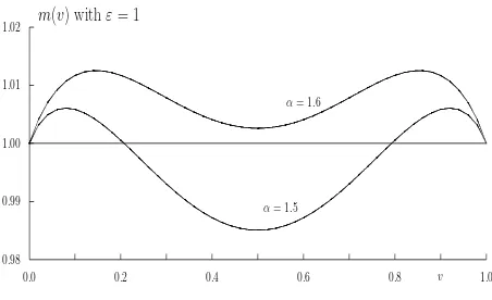
ǫ=1. Forα≤1, the setA0is empty. Forα=α0=log 3/log 2≈1.585,A0= (0, 0.5)∪(0.5, 1). For
1< α < α0,A0consists of two smaller separated intervals. Forα > α0, we haveA0= (0, 1)(see Fig.
4). Again Theorem 2 can be applied with the same behavior of the trajectories as in Example 2.
0.0 0.2 0.4 0.6 0.8 v 1.0
0.98 0.99 1.00 1.01
1.02 m(v) withε= 1
α= 1.5
α= 1.6
1
Figure 4: Conditional mean functionm(v)for example 3 withα=1.5 and 1.6, withǫ=1.
3
Overview on the proofs
The proof of the two results is rather lengthy and technical. Therefore, we indicate the basic ideas of the proof first without much technicalities. The applied ideas of the two proofs are the same. For the double cluster events with the path behavior given bym(v), one can consider the Gaussian process
(X(s),X(t))on[0,T]2. The events which contribute mostly to the asymptotic probability, are those with time points(s,t)∈D={(s,t):|t−s−tm| ≤δ}for some positiveδ. This domain is then split into smaller two-dimensional ’intervals’∆k×∆l of suitable lengthλu−2/α (for someλ >0) in case of Theorem 1, and another length in Theorem 2. The probability of such double exceedance clusters and exceedance behavior in the small ’intervals’ are derived asymptotically exact for the two cases assumingC2orC3. These results are given in Lemma 1 and Lemma 2. Their proofs are combined because a good part follow the same steps where we condition on the event{X(s)> u,X(t)>u}
fors,t in the subinterval separated byτwhich is neartm. Here we have to consider the conditional process converging to the limit process which defines also the Pickands type conditions. The limit is holding using a domination argument.
The Pickands type constants are considered in Lemma 4 and 5 where neighboring and separated intervals are considered. Further properties for these constants are investigated in Lemma 7 and 8.
The proof of Theorem 1 is given in Section 4 which follows the ideas mentioned above, dealing with the double exceedance clusters inDand outsideD, showing that a double exceedance cluster occurs with much smaller probability than within D, which gives the presented result. For the domain D
with the subintervals we apply Lemma 1. The lower bound needs again Lemma 1, but also the results in Lemma 8. The proof of the second statement of Theorem 1 is much simpler.
Similar ideas are applied in the proof of Theorem 2 based on different intervals. We have to consider the three casesα >1,=1 and<1 separately since the path behavior of the conditioned Gaussian process plays a role. This is similar (but technically more complicated) to Theorem D.3 in[8], when different relations between smoothness of trajectories and smoothness of variance in its maximum point lead to quite different type of considerations.
We note that limiting conditioned processes are fractional Brownian motions with trend, where the Brownian motions have positive dependent increments ifα >1, independent increments ifα=1, and negative correlated increments ifα <1. The major contribution to the asymptotic probability comes in all three cases from events whereX(s)>u,X(t)>uwiths,t separated by not more than ǫ+o(1) (with o(1) →0 as u→ ∞). Again we apply subintervals and the Bonferroni inequality, with the double sum method for the lower bounds where the subintervals are adapted to the three different cases ofα. In all four cases considered by Theorems 1 and 2, one has to choose the lengths of the two-dimensional small intervals carefully in Lemma 1 and 2, to hold the double sum infinitely smaller than the sum of probabilities in the Bonferroni inequality. The cases of Theorem 1 and Theorem 2 (iii) are similar because the smoothness of the variance exceeds the smoothness of the trajectories. Therefore, we choose the same two-dimensional ’subintervals’ and prove these cases in the same way.
The second part of Theorem 2 is as for the second statement of Theorem 1, and is not repeated.
4
Lemmas
We writeaΛ ={a x : x∈Λ}and(a1,a2) + Λ ={(a1,a2) +x : x∈Λ}, for any real numbersa,a1,a2
and setΛ⊂R2. LetAbe a set inR, andAδ:={t: infs
∈A|t−s| ≤δ}itsδ-extension, withδ >0. We denote the covariance matrix of two centered random vectorsU,Vby
cov(U,V) =EUVT
and
cov(U) =E(UUT).
In the following, we letτbe a point in[0,T]which may depend onuand lies in the neighborhood of
tm where r(τ)is either twice continuously differentiable (in case of ConditionC2) or continuously differentiable (in case of ConditionC3withtm=ǫ).
Lemma 1 and 2 deal with the events of interest on small intervals assuming the conditionC2and
C3, respectively. Here the limiting conditioned process enters with the Pickands type conditions. For
S∈ S andΛ⊂R2, denote
p(u;S,Λ):=P
[
(s,t)∈(0,τ)+u−2/αΛ
{X(s)>u,X(t)>u,TsS}
Lemma 1. Let X(t) be a Gaussian process with mean zero and covariance function r(t) satisfying assumptionsC1andC2. LetΛbe a closed subset ofR2.
(i) Then for anyτ=τ(u)with|τ−tm|=O(u−1plogu)as u→ ∞,and any S∈ S0,
p(u;S,Λ)∼hα
Λ
(1+r(tm))2/α
Ψ2(u,r(τ)), (4)
as u→ ∞, where
hα(Λ) =
Z ∞
−∞
Z ∞
−∞
ex+yP
[
(s,t)∈Λ
(p2Bα(s)− |s|α>x,
p
2 ˜Bα(t)− |t|α> y)
d x d y,
with Bα, ˜Bα are independent copies of the fractional Brownian motion with the Hurst parameterα/2.
In particular, forΛ1andΛ2,closed subsets ofR,
p(u;S,Λ1×Λ2)∼Hα,0
Λ1
(1+r(tm))2/α
Hα,0
Λ2
(1+r(tm))2/α
Ψ2(u,r(τ)) (5)
as u→ ∞.
(ii) Further, for any S∈ S1there exist C>0,δ >0such that
p(u;S,Λ)≤C e−δu2Ψ2(u,r(τ)). (6)
Remark 3: Note that if|τ−tm|=o(u−1), thenΨ2(u,r(τ))∼Ψ2(u,r(tm))asu→ ∞.
Lemma 2. Let X(t) be a Gaussian process with mean zero and covariance function r(t) satisfying
assumptionsC1andC3withα≤1. LetΛbe a closed subset ofR2.
(i) Letτ=τ(u),be such that|τ−ǫ|=O(u−2logu)as u→ ∞. Then for any S∈ S0andα <1,
p(u;S,Λ)∼hα
Λ
(1+r(ǫ))2/α
Ψ2(u,r(τ)) (7)
as u→ ∞. Ifα=1, (7) holds with hα replaced by
˜h
1(Λ) =
Z ∞
−∞
Z ∞
−∞
ex+yPn [
(s,t)∈Λ
(p2B1(s)− |s| −r′(ǫ)s>x,
p
2 ˜B1(t)− |t|+r′(ǫ)t> y)od x d y
(ii) Statement(ii)of Lemma 1 holds also in this case.
Proof of Lemma 1 and 2: The proofs of both lemmas can be derived partially together with the
same steps, where it does not matter whether tm is an inner point or the boundary pointǫ. Some deviations are induced by this difference oftm, hence with different smoothness conditions around
denoted by ’Part for Lemma 1’ and ’Part for Lemma 2’. If both cases can be dealt with together, we denote the paragraph as ’Common part’.
Statement (i): Common part: Let S ∈ S0 which means that there are closed sets A⊂ A0 and
B⊂B0. Obviously, r(t)>−1 in a neighborhood of tm. We have for anyu>0, denoting for short,
K= (0,τ) +u−2/αΛand
U(K,S) =[(s,t)∈K{X(s)>u, X(t)>u,TsS},
p(u;S,Λ) =u−2
Z Z
P
U(K,S)| X(0) =u− x
u, X(τ) =u− y u
×fX(0),X(τ)(u− x u,u−
y
u)d x d y. (8)
Consider first the conditional probability in (8). Denote by Px,y the family of conditional probabili-ties givenX(0) =u−ux, X(τ) =u− uy. Letκ >0 be small such that theκ-extensions ofAandB are still subsets ofA0andB0, respectively,Aκ⊂A0,Bκ⊂B0, then the corresponding eventSκ∈ S0, and
for all sufficiently largeuand all(s,t)∈K,Sκ⊂TsS. Note thatSκ is independent ofs, if(s,t)∈K. Hence
U(K,S)⊇Sκ∩
[
(s,t)∈K{X(s)>u, X(t)>u}=Sκ∩U(K,Ω).
Now we prove thatPx,y(Sκ∩U(K,Ω))∼Px,y(U(K,Ω))asu→ ∞. For the conditional mean ofX(v), using inequality(r(s)−r(t))2≤2(1−r(t−s))and the conditions of the two lemmas, we have by
simple algebra,
Mx y(v,u):=E
X(v)
X(0) =u− x
u, X(τ) =u− y u .
=(u−x/u)(r(v)−r(τ−v)r(τ)) + (u−y/u)(r(τ−v)−r(v)r(τ))
1−r2(τ)
=ur(v) +r(τ−v)
1+r(τ) +
1
u(g1(v,τ)x+g2(v,τ)y)
=um(v)1+Ou−α(logu)α/2+O(u−1)(g1(v,tm)x+g2(v,tm)y),
where g1 and g2 are continuous bounded functions. The conditional variance can be estimated as follows,
Vx,y(v):=var(X(v)|X(0),X(τ)) = det cov(X(0),X(τ),X(v))
1−r2(τ) ≤1. (9)
We have by the construction ofSκ, infv∈Aκm(v)>1 and supv∈Bκm(v)<1. Similarly as (9), we get
that
Vx,y(v,v′):=var(X(v)−X(v′)|X(0),X(τ))≤var(X(v)−X(v′))≤C|v−v′|α.
Hence there exists an a.s. continuous zero mean Gaussian process Y(v) with variance V(v) and variance of increments V(v,v′). Using Fernique’s inequality and (9), for any positive δ1 <
min(minv∈A
κm(v)−1, 1−maxv∈Bκm(v)), we derive for all sufficiently largeu,
Px,y U(K,Ω)\Sκ≤Px,y Ω\Sκ ≤min(P(inf
v∈Aκ
Y(v) +Mx y(v,u)<u),P(sup v∈Bκ
Y(v) +Mx y(v,u)>u)
which gives the desired result
Px,y(U(K,S))≥Px,y Sκ∩U(K,Ω)
≥Px,y(U(K,Ω))−Cexp(−δ12u
2/2). (10)
Notice that also
Px,y(U(K,S))≤Px,y(U(K,Ω)). (11) Now we study the integrand in (8) replacingPx,y(U(K,S))byPx,y(U(K,Ω)). To this end we consider the limit behavior of the conditional distributions of the vector process(ξu(t), ηu(t)), where
ξu(t) =u(X(u−2/αt)−u) +x, ηu(t) =u(X(τ+u−2/αt)−u) + y,
given(ξu(0),ηu(0)) = (0, 0) (that isX(0) = u−x/u, X(τ) =u−y/u). These Gaussian processes describe the cluster behavior which are separated by at leastǫ. We need to know the mean and the covariance structure ofξu(s)andηu(s)with the limiting expressions for the corresponding limiting processesξ(s)andη(s). We have,
E
ξu(t) ηu(t)
ξu
(0)
ηu(0)
=E
ξu(t) ηu(t)
+RtR−01
ξu(0)−Eξu(0) ηu(0)−Eηu(0)
, (12)
where
Rt:=E
ξu(t)−Eξu(t) ηu(t)−Eηu(t)
ξu(0)−Eξu(0) ηu(0)−Eηu(0)
⊤!
.
Further,
Eξu(0) =Eξu(t) =x−u2, Eηu(0) =Eηu(t) = y−u2, (13)
varξu(0) =varηu(0) =u2, cov(ξu(0),ηu(0)) =u2r(τ), cov(ξu(0),ξu(t)) =cov(ηu(0),ηu(t)) =u2r(u−2/αt),
cov(ξu(0),ηu(t)) =u2r(τ+u−2/αt), cov(ξu(t),ηu(0)) =u2r(τ−u−2/αt). (14) We write
r(u−2/αt) =1−u−2|t|α+o(u−2),
r(τ±u−2/αt) =r(τ)±u−2/αt r′(τ+θ±u−2/αt), where|θ±| ≤1. Obviously, ifα <1, it follows for both lemmas, that
r(τ±u−2/αt) =r(τ) +o(u−2). (15)
Part for Lemma 1:For this lemma the last relation (15) also holds forα∈[1, 2)by using|τ−tm|=
O(u−1plogu). Indeed, we get|r′(τ+θ±u−2/αt)−r′(tm)|=O(u−1 p
logu)and againr(τ±u−2/αt) = r(τ) +o(u−2). This implies that with the notationr=r(τ)andr′=r′(τ)
Rt=u2
1−u−2|t|α+o(u−2) r+o(u−2) r+o(u−2) 1−u−2|t|α+o(u−2)
whereI denotes the identity matrix. Note that
Common part: Since the conditional expectation is linear, the o(1) terms in (16), (17) have the
is the matrix of covariances of the two random vectors. Then, asu→ ∞,
var(ξu(t)−ξu(s)) =var(ηu(t)−ηu(s)) =2u2(1−r(u−2/α(t−s)))∼2|t−s|α (19)
Part for Lemma 1: Using the Taylor expansion, we get by C2asu→ ∞
cov(ξu(t)−ξu(s),ηu(t1)−ηu(s1))
=u2(r(τ+u−2/α(t1−t)) +r(τ+u−2/α(s1−s))−r(τ+u−2/α(t1−s))
−r(τ+u−2/α(s1−t)))
=u2(u−2/αr′(τ)(t1−t+s1−s−t1+s−s1+t+O(u−4/α))
=O(u2−4/α) =o(1) (20)
Part for Lemma 2: In this case the second derivative is not used. Sinceα≤1, the statement holds
in the same way byC3.
cov(ξu(t)−ξu(s),ηu(t1)−ηu(s1))
=u2(u−2/αr′(τ)(t1−t+s1−s−t1+s−s1+t) +o(u−2)) =o(1). (21)
Common Part:Further we have for both lemmas,
cov(ξu(t)−ξu(s),ξu(0)) =cov(ηu(t)−ηu(s),ηu(0)) =u2(r(tu−2/α)−r(su−2/α)) =O(1),
cov(ξu(t)−ξu(s),ηu(0)) =u2(r(τ−u−2/αt)−r(τ−u−2/αs)) =O(u2−2/α), cov(ηu(t1)−ηu(s1),ξu(0)) =O(u2−2/α),
so each element of the matrix
Ccov
ξu(0) ηu(0)
−1
C⊤
is bounded by
O(u4−4/α) u2 =O(u
2−4/α) =o(1) (22)
asu→ ∞. This implies together that (18) can be written as
cov
ξu(t)−ξu(s) ηu(t1)−ηu(s1)
ξu
(0)
ηu(0)
=
2|t−s|α 0 0 2|t1−s1|α
(1+o(1))
asu→ ∞. Since the conditional variance is bounded by the unconditional one, we get that
var(ξu(t)−ξu(s)|ξu(0),ηu(0))≤C|t−s|α, (23)
var(ηu(t)−ηu(s)|ξu(0),ηu(0))≤C|t−s|α, (24)
for all t,s ∈ [0,∞). Thus we proved that for any T > 0, the distribution of the Gaussian vector process (ξu(t),ηu(t)) conditioned on ξu(0) = ηu(0) = 0 converges weakly in C[−T,T] to the distribution of the Gaussian vector process(ξ(t),η(t)), t∈[−T,T]. This implies that
lim
u→∞Px,y(U(K,Ω)) =P
[
(s,t)∈Λ
{ξ(s)>x, η(t)> y}
Furthermore, we have forξandηthe following representations:
Part for Lemma 1: The limit process are
ξ(t) =p2Bα(t)− |t|
Part for Lemma 2: The limit processes are
ξ(t) =p2Bα(t)−
Common Part: Domination:We want to apply the dominated convergence theorem for the integral
in (8) divided byΨ2(u,r), hence to
We construct an integrable dominating function with separate representations in the four quadrants as follows. Use (11) and bound the probabilityPx,y(U(K,Ω)). LetT>0 be such thatΛ⊂[−T,T]×
and the function fu by
exp
for sufficiently large u, using arguments similar to 1. The function pu(x) can be bounded by
Cexp(−b x2), b>0, using the Borel inequality with relations (16) - (24). Similar arguments were applied in Ladneva and Piterbarg[4].
Again, in the same way we apply the Borel inequality for the probability, to get the bound
Cexp(−b(x+y)2), with a positiveb.
The four bounds give together the dominating function for the integrand in (25).
Asymptotic probability: Finally we transform the limit of (25) using the self-similarity of the
frac-tional Brownian motion. We give the transformation for Lemma 1 with ˜r=r(tm). The correspond-ing transformation for Lemma 2 withα <1 and ˜r = r(ǫ) is the same and for α= 1 it is similar.
This shows first statements of the two lemmas.
Statement (ii): It remains to prove the statements (ii) of both lemmas, it means the bound (6).
SinceS ∈ S1, the setAcontains an inner point v∈B0 or B contains an inner pointw ∈A0. In the
We have for all sufficiently largeuthat with its minimal point at
Chooseεsmall such that
δ1=
(1−m(v))2
1+b2(tm)−2m(v)
−ε >0.
Since the Gaussian field Y(s,t) satisfies the variance condition of Theorem 8.1 of [8], we can use this inequality result to get that
Pu,S≤Cucexp
− u
2
(1+r(tm))(1−δ1)
,
for some positive constants C and c. This implies that the statements of the lemmas hold for the first probability of (27) for any positiveδ < δ1/(1+r(tm)).
Now we turn to the second probability term in (27) withw such thatm(w)>1. We estimate the probability in the same way from above again with any ˜α >0.
P(u,S,Λ)≤P
X(w)≤u, [
(s,t)∈(0,τ)+u−2/αΛ
{X(s)>u,X(t)>u}
≤P X(w)≤u, sup
(s,t)∈(0,τ)+u−2/αΛ
(X(s) +X(t))>2u
!
P −α˜X(w)≥ −α˜u, sup
(s,t)∈(0,τ)+u−2/αΛ
(1+α˜)b−1X(s,t)>(1+α˜)u
!
≤P sup
(s,t)∈(0,τ)+u−2/αΛ−
˜
αX(w) + (1+α˜) X(s,t) b(t−s) >u
! .
The variance of the fieldY(s,t) =−α˜X(w) + (1+α˜)X(s,t)
b(t−s) equals
˜
α2+b−2(1+α˜)2−2 ˜α(1+α˜)b−2m = b−2((b2+1−2m)α˜2−2(m−1)α˜+1).
Notice that for anys,t,w, we haveb2+1−2m>0, otherwise we would have a negative variance. The minimum of the parabola is at
˜
α= m−1
b2+1−2m>0
for all sufficiently largeu,, with value
D2s,t(v):= 1 b2(t−s)
1− (ms,t(w)−1)
2
1+b2(t−s)−2m s,t(w)
.
By the same steps as above, the stated bound holds again for the second probability of (27), which
show the second statements of both lemmas.
Corollary 3. For anyα∈(0, 2),anyΛ>0andτas in Lemma 1, the sequence of Gaussian processes
ξu(s)−E˜ξu(s)andηu(t)−E˜ηu(t)conditioned onξu(0) =ηu(0) =0converges weakly in C[−Λ,Λ]
to the Gaussian processesp2Bα(s)and
p
2eBα(t)),respectively, as u→ ∞.
Indeed, to prove this we need only relations (18, 19, 22) with (23, 24), which are valid by the assumptions of the corollary.
The following lemma is proved in Piterbarg[8], Lemma 6.3, for the multidimensional time case. We formulate it here for the one-dimensional time where we consider the event of a double exceedance separated byC(u−2/α)for some constantC>0.
Lemma 3. Suppose that X(t)is a Gaussian stationary zero mean process with covariance function r(t)
satisfying assumptionC1. Letεwith be such that 1
2 > ε >0and
1−1
2|t|
α
≥r(t)≥1−2|t|α
for all t∈[0,ǫ]. Then there exists a positive constant F such that the inequality
P
The following two lemmas are straightforward consequences of Lemma 6.1, Piterbarg [8] giving the accurate approximations for probabilities of exceedances in neighboring intervals or of a double exceedance in neighboring intervals.
Lemma 4. Suppose that X(t)is a Gaussian stationary zero mean process with covariance function r(t)
satisfying assumptionC1. Then for anyλ,λ0>0,
Lemma 5. Suppose that X(t)is a Gaussian stationary zero mean process with covariance function r(t)
Proof. Write
P
max
t∈[0,λu−2/α]X(t)>u,t∈[λ max
0u−2/α,(λ0+λ)u−2/α]
X(t)>u
=P
max
t∈[0,λu−2/α]X(t)>u
+P
max
t∈[λ0u−2/α,(λ0+λ)u−2/α]
X(t)>u
−P
max t∈[0,λu−2/α]∪[λ
0u−2/α,(λ0+λ)u−2/α]
X(t)>u
and apply Lemma 6.1, Piterbarg[8]and Lemma 4.
From Lemmas 5 and 3 we get a bound forHα([0,λ],[λ0,λ0+λ]), the Pickands type constant, which
depends on the separationλ0−λ.
Lemma 6. For anyλ0> λ,
Hα([0,λ],[λ0,λ0+λ])≤F
p
2πλ2e−18(λ0−λ)α.
Whenλ0 = λthe bound is trivial. A non-trivial bound for Hα([0,λ],[λ, 2λ])is derived from the
proof of Lemma 7.1, Piterbarg [8], see page 107, inequality (7.5). This inequalitiy, Lemma 6.8, Piterbarg[8]and Lemma 3 give the following bound.
Lemma 7. There exists a constant F1 such that for allλ≥1,
Hα([0,λ],[λ, 2λ])≤F1
p
λ+λ2e−18λ
α
.
Applying the conditioning approach of Lemmas 1 and 2 to the following event of four exceedances, we can derive the last preliminary result by usingHα(·)of Lemma 5.
Lemma 8. Let X(t) be a Gaussian process with mean zero and covariance function r(t)withα <1,
satisfying assumptionsC1and eitherC2orC3. Letτ=τ(u)satisfies either the assumptions of Lemma 1 or the assumptions of Lemma 2. Then for allλ >0,λ1≥λ,λ2≥λ
P
max
t∈[0,u−2/αλ]X(t)>u,t∈[u−2/αλmax
1,u−2/α(λ1+λ)]
X(t)>u,
max
t∈[τ,τ+u−2/αλ]X(t)>u, t∈[τ+u−2/αλmax
2,τ+u−2/α(λ2+λ)]
X(t)>u
= Y
i=1,2
Hα [0,κλ],
κλi,κ(λi+λ)
Ψ2(u,r(τ))(1+o(1)),
as u→ ∞, whereκ= (1+r(tm))−2/α.
5
Proof of Theorem 1
First part:
DenoteΠ ={(s,t):s,t∈[0,T]and t−s≥ǫ},δ=δ(u) =Cplogu/u, where the positive constant
C is specified later, andD={(s,t)∈Π: |t−s−tm| ≤δ}.
a) We want to show that we have to deal mainly with the domainD, since events occuring outside ofDoccurs with asymptotically smaller probability. We have for anyS∈ S0,
Pǫ,u,T(S)≤P
and on the other hand, for all sufficiently largeu,
Pǫ,u,T(S)≥P
The second term of the right-hand side of (28) is bounded by
P
Making use of Theorem 8.1, Piterbarg[8], we can bound the last probability by
const·u−1+2/αexp
For all sufficiently largeu, the maximal correlation onΠ\Dis bounded by
max
(s,t)∈Π\Dr(t−s)≤r(tm)−0.4|r
′′(t
m)|δ2(u) =r(tm)−0.4C2|r′′(tm)|u−2logu. Hence, the second term is of smaller order than the leading term, since
P
b) Now we deal with the first probability in the right-hand side of (28), with events occuring in
D. We bound the probability from above and from below such that the bounds are asymptotically equivalent. Denote∆ =λu−2/α, for someλ >0, and define the intervals
where[·]denotes the integer part. We will apply Lemma 1 for sets∆k×∆l = (0,(l−k)∆)+∆k×∆k, Using this, we can approximate the sumΣ1 by an integral
using the definition ofΨ(u,r)
this bound gives asymptotically the asymptotic term of Theorem 1.
We choose the value ofC. LetC be so large thatG>2−2/α, which implies that the left-hand side of (30) is infinitely smaller than the left-hand side of (34), asu→ ∞.
c) We bound now the probability in the right-hand side of (29) from below. By the Bonferroni inequality we get
where second term, the double sum, has been increased by omitting the eventsTsS. This double-sum in (35) is taken over the set
K={(k,l,k′,l′): (k′,l′)6= (k,l),∆k×∆l ⊂D, ∆k′×∆l′⊂D}.
The first sum in the right-hand side of (35) can be bounded from below in the same way as the previous sum in (32), therefore it is at least the right-hand side of (34) with a change of(1+γ2(u))
by(1−γ2(u)).
Consider the double-sumΣ2, say, in the right-hand side of (35). For simplicity we denote
H(m) =Hα,0
With Lemma 8 we derive for the probability
with k ≤ k′, l ≤ l′, takingλ1 = (k′−k)λ, λ2 = (l′−l)λ, andτ = (l−k)∆. Note that τ→ tm uniformly for the possiblekandl. Since the processX is stationary, we have for the double-sumΣ2
in (35) (which includes only different pairs(k,l)and(k′,l′)) withL={k≤k′,l≤l′,(k,l)6= (k′,l′)} do not depend onkandl. The last sum was considered already in (33).
d) Hence, it remains to bound the sum ofH(n). By (5), (6) and (7) and Lemma 6.8 of Piterbarg
which shows that the double-sumΣ2 is infinitely smaller than (34) or the asymptotic term of the statement, lettingλ→ ∞. Thus the first assertion of Theorem 1 follows.
Second part:
Finally we turn to the second assertion of Theorem 1, whereS∈ S1. By Lemma 1, each term in the sum (31) can be bounded uniformly by
exp{−δu2}Ψ2(u,r(tm)),
for all sufficiently largeu, where δ >0. Since the number of summands in (31) is at most a power
ofu, the statement of Theorem 1 follows.
6
Proof of Theorem 2.
We begin with the proof of the first part of Theorem, assumingS ∈ S0, dealing separately with the
6.1
Proof of Theorem 2(i).
In this caseα >1. Letb≥a, introduce the event
Uu;a,b,T(S):={∃(s,t): s,t∈[0,T], b≥t−s≥a, X(t)≥u, X(s)≥u,TsS}, withUu;a,b,T :=Uu;a,b,T(Ω). In particular, for anyS, P(Uu;ǫ,b,T(S)) =Pu;ǫ,T(S)for allb≥T, and
P(Uu;ǫ,ǫ,T(S)) =P(∃t∈[ǫ,T]:X(t−ǫ)∧X(t)>u,Tt−ǫS).
Letδ(u) =cu−2logu,c>0, andγ >0 a small positive number. Then for allusuch thatδ(u)≥γu−2, (which holds forusuch that logu≥γ/c ),
Uu;ǫ,T,T(S)⊆Uu;ǫ,T,T
⊆Uu;ǫ,ǫ+γu−2,T∪(Uu;ǫ+γu−2,ǫ+δ(u),T \Uu;ǫ,ǫ+γu−2,T)∪Uu;ǫ+δ(u),T,T (36)
and
Uu;ǫ,T,T(S)⊇Uu;ǫ,ǫ+γu−2,T(S)⊇Uu;ǫ,ǫ,T(S). (37)
We estimate from above the probabilities of the third and second event in the right-hand side of (36). Then we derive the asymptotic behavior of the probability of the first event in the right-hand side with smallγand show that it dominates the two other ones. Finally, we need to estimate the probability of the event in the right hand part of (37) from below, and show that it is equivalent to the upper bound.
6.1.1 Large separation of the clusters
We estimate from above the probability of the third event in the right-hand side of (36). Using the inequality of Theorem 8.1,[8], with r(t) < r(ǫ+δ(u))for t > ǫ+δ(u) by C3, we get with
r=r(ǫ),r′=r′(ǫ)
P(Uu;ǫ+δ(u),T,T)
≤P(∃(s,t): s,t∈[0,T], t≥s+ǫ+δ(u), X(t) +X(s)>2u)
=P
max
s,t∈[0,T],t≥s+ǫ+δ(u)(X(t) +X(s))>2u
≤Cu4/α−1exp
− u
2
1+r(ǫ+δ(u))
≤Cu4/α−1exp
− u
2
1+r +
u2δ(u)r′(1+o(1)) (1+r)2
≤Cu−Rexp
− u
2
1+r
, (38)
for anyR>0 by choosingc inδ(u)sufficiently large, with some constantC>0, sincer′<0. This estimate holds for anyα≤2.
6.1.2 Intermediate separation of clusters
Now we estimate the probability of the second event in the right-hand side of (36). We have
P(Uu;ǫ+γu−2,ǫ+δ(u),T\Uu;ǫ,ǫ+γu−2,T)≤P(Uu;ǫ+γu−2,ǫ+δ(u),T ∩Uc
For any positive gwithg< γ, we use time points on the gridk gu−2 to estimate
withξu(s) = u(X(u−2/αs)−u) +x andηu(t) = u(X(τ+u−2/αt)−u) + y. Now we estimate the
for anya∈(0, 1)and all sufficiently largeu. Similar to the derivation in Lemma 2, the conditional variance of the increments is bounded by the unconditional variance of the increments and the process converges asu→ ∞, see Corollary 3. We have therefore,
e
By symmetry, the same is valid forp2by using (41), thus we have shown that
lim
First we study the conditional means and covariance functions of the process
given (ξu(0),ηu(0)) = (0, 0). Note that another time scaling is used, u−2, instead of u−2/α as in thus the elements ofΣare bounded, which implies
Σcov any non-negative integermwe have
where we use the stationarity and the domination, as in the proof of Lemma 2. The probability has been changed to the indicator function in view of the deterministic limiting behavior. Denoting δ1 =γ|r′|/(1+r)2, L1 = L|r′|/(1+r)2 and changing variables ˜x = x/(1+r), ˜y = y/(1+r), ˜t =
t|r′|/(1+r)2and ˜s=s|r′|/(1+r)2, we get Z Z
{∃(s,t):t−s∈[0,γ],s∈[0,L],−r′s/(1+r)>x,r′t/(1+r)>y} exp
x+y
1+r
d x d y
= (1+r)2
Z Z
{∃(˜s,˜t):˜t−˜s∈[0,δ1], ˜s∈[0,L1], ˜s>˜x,−˜t>˜y},˜x≤0
exp(˜x+ ˜y)d˜x d˜y
+ (1+r)2
Z Z
{∃(˜s,˜t):˜t−˜s∈[0,δ1], ˜s∈[0,L1], ˜s>˜x,−˜t>˜y},˜x>0
exp(x˜+˜y)d˜x d˜y
≤(1+r)2
Z0
−∞
Z 0
−∞
exp(˜x+˜y)d˜x d˜y+
Z L1
0
Z −˜x
−∞
exp(˜x+˜y)d˜x d˜y
!
= (1+r)2(1+L1) = (1+r)2+L|r′|. (44)
since ˜t≥˜s≥˜x. Similar to Section 3.1.2 we get
P(Uu;ǫ,ǫ+γu−2,T)≤
T−ǫ+o(1)
Lu−2 P0
∼ T−ǫ
Lu−2
exp−u2/(1+r)
2πu2p1−r2
(1+r)2+L|r′|,
and
lim sup L→∞
lim sup u→∞ P
(Uu;ǫ,ǫ+γu−2,T)exp
u2/(1+r)≤ (T−ǫ)|r ′|
2πp1−r2
. (45)
It remains to derive a lower bound of the probability of right hand part of (37). Using stationarity we write
P(Uu;ǫ,ǫ+γu−2,T(S))≥P(Uu;ǫ,ǫ,T(S))
≥ T−ǫ
Lu−2
p0(S)−
[(T−ǫ)Xu2/L]+1
m=1
p0,m
, (46)
where
p0(S) =P(∃t:t∈[0,Lu−2]:X(t)≥u,X(t+ǫ)≥u,TtS),
p0,m=P(∃(s,t): s∈[0,Lu−2], t∈[mLu−2,(m+1)Lu−2]:
Further, with someA⊂A0 andB⊂B0 (47). We have byC1, for all sufficiently largeu,
sup
One may select d = ˜cu1−α since α >1, with sufficiently large ˜c such that the above probability is smaller than exp−1+2ur2(ǫ), for all sufficiently large u. The same is valid for the difference
probabilities is based on the same methods as for the proof of Lemma 2. The first probability equals
1
above conditional probability is uniformly greater than one andd →0, the probability contributes exp−au˜2 with some a > 0. Thus the probability has order exp−1+bur(ǫ)2 with some b > 1. Similarly for the second probability, since the conditional mean onBlu−2 is uniformly less than one.
Together, the second term of the right hand side of (47) is at most of the same order, and of smaller order than (48).
The above right-hand side can be bounded similarly to the derived bound ofPm(see (44) and (45)), but by usingτ=ǫ+mLu−2 instead ofǫ. We have,