CONSTRUCTING EARLY WARNING SYSTEM OF CURRENCY
CRISES FOR INDONESIA: Leading Indicator Approach
By Eric Alexander Sugandi*)
A b s t r a c t
Krisis mata uang pada periode 1997-1999 lalu merupakan shock terbesar yang dialami oleh perekonomian Indonesia. Krisis ini memporak-porandakan perekonomian ditandai dengan penurunan pertumbuhan yang tajam dan tercabiknya sistem perbankan. Jika otoritas moneter dan pelaku bisnis mampu mengantisipasi krisis mata uang ini, kita dapat berharap kerugian sosial lebih kecil. Belajar dari kesalahan masa lalu, sangat penting untuk membangun early warning system yang dapat memprediksi kemungkinan terjadi krisis mata uang.
Studi ini mempergunakan pendekatan leading indicator untuk membangun early warning sys-tem atas krisis mata uang di Indonesia. Krisis mata uang didefinisikan sebagai setiap bentuk tekanan atas nilai tukar (EMP) baik dalam level maupun variasinya. Setiap kinerja indikator diukur dengan mempergunakan tiga kriteria: 1. Persentage kebenaran klasifikasi, 2. Adjusted noise to signal ratio, 3. Probabilita terjadinya krisis mengikuti signal.
Hasil dari studi ini menunjukkan bawa ada lima indikator terbaik yang memenuhi seluruh kriteria, yakni: 1) Misallignment nilai tukar riil rupiah disekitar nilai trend, 2. Pertumbuhan foreign asset dari Deposit Money Bank, 3) Surplus neraca keuangan, 4) Pertumbuhan base money, dan 5) Ratio sur-plus neraca keuangan terhadap GDP. Dari indikator individual terbaik, kita dapat membuat 17 indikator komposit terbaik. Diantara semua indikator, yang paling unggul adalah “VW”, kombinasi langsung antara point 1 dan 2.
Source: Bloomberg
0 2000 4000 6000 8000 10.000 12.000 14.000 16.000 18.000
Jan Mar Mei Jul Sep Nov Jan Mar Mei Jul Sep Nov Jan
1997 1998 1999
1. Introduction
The 1997-1999 currency crises series, which began in August 1997, was an
unanticipated major shock to Indonesian economy. All in a sudden,Indonesia became one
among victims of contagious currency crises across Asia Pacific. Starting from Thailand in
June 1997, followed by the Philippines and South Korea, currency crises disease finally
grabbed Indonesia.
Many financial institutions in Indonesia, either domestic or foreign institutions, had
failed to predict the occurence of the crisis. In fact, these institutions were very optimitic in
jugding the performance of Indonesian economy, and even some analysts believed that
Indonesia would not suffer currency crisis as happened in other Asian countries. The
Jakarta Composite Index (JCI) reached its peak (740.8) on 8th July 1997, only six days
after Thailand abandoned its fixed exchange rate regime. Meanwhile, country risk for
interest rate did not change significantly, reflecting market optimism to Indonesia’s resilience
toward crisis attack.
Indonesia’s economic condition turned bad as Bank Indonesia failed to stabilize Rupiah.
In July 1997, Rupiah was depreciated by 0.2% toward US Dollar from its average exchange
rate in June 1997. On 11th June 1997, Bank Indonesia widened the exchange rate band
from 8% to 12%, but this effort was fruitless. Compared to the average exchange rate of
Rupiah to US Dollar in June 1997, Rupiah had dropped by 12.6% in August, 19.9% in
September, 32.3% in October, 29.9% in November, and 50.2% in December 1997.
Facing currency crisis, Foreign Direct Investment (FDI) and portfolio investment to
Indonesia saw significant declines in the third and fourth quarter of 1997, and even fell to
negative values. Demand for US dollar sharply increased as foreign investors tried to minimize
their loss by expediting their payment of foreign currency debts. Meanwhile, speculators
tried to gain profit by trading foreign currencies, mainly the US Dollar. As a consequence of
these simultaneous attacks, Rupiah sunk further.
In general, it can be concluded that most financial institutions in Indonesia were
failed to anticipate the 1997-1999 currency crises series. Learning from past failures in
anticipating currency crises, many economists have tried to develop early warning system
to deal with the possibility of currency crisis ocurrence in the future. The system will be
very useful if it can prevent policy makers and business practitioners from severe losses
caused by crisis.
This study is an attempt to develop early warning system for Indonesia. Unlike some
previous early warning system studies (which use panel data of many countries accross the
time, or time series data of a single country other than Indonesia), this study uses Indonesian
time series data only. It is expected that this study will capture special characteristics of
Indonesian economy, that cannot be revealed by panel data nor by other-country single
data studies.
2. Purpose of Study and Hypothesis
The purpose of this study is to construct early warning system of currency crises for
Indonesia. The early warning system should be useful to predict possibility of currency
crises occurrence in the future. In order to achieve this big goal, two smaller objectives are
involved:
1) Constructing early warning system of currency crises models. Individual leading indicators
and composite leading indicator models are the focus in this study, hence they are
constructed to be ready-to-use early warning system models.
2) Determining robust variables in all models, which will be useful for further early warning
system development. These variables should be best individual leading indicators and
become elements of the best composite leading indicators.
The hypothesis behind this study is that there are some variables, among all variables
in examination, which perform as best individual indicators to predict currency crisis
occurrence in the near future. Some of these variables may also serve as elements of the
3. Currency Crisis and Its Causes
Prior to further discussion about early warning system models, it is better to understand
“currency crisis” and its causes. In general, “currency crisis” is defined as a condition where
extraordinary exchange market pressure abruptly changes existing exchange rate level to a
new one, with relatively high difference between the previous and the new exchange rate.
In many literatures, “currency crisis” term refers only to a currency devaluation or depreciation
against other currency. From literatures reviewed in this study, at least four factors can be
considered as causes of currency crisis: (1) excessive monetary policy and domestic credit
expansion; (2) current account deterioration; (3) financial system fragility; and (4) high
degree of economic openness toward foreign exposures.
Kaminsky, Lizondo, and Reinhart (1998) classified currency crisis models based on
the two earliest factors as models with “traditional approach”. In traditional approach models,
significant changes in macroeconomic fundamentals are main causes of currency crisis.
Models based on the third factor belong to “recent (approach) models”. In recent approach
models, currency crisis can occur with or without any significant changes in economic
fundamentals, since interaction between economic agents’ and government’s expectations
becomes the driving force that generates speculative attack to a currency. The last factor is
derived from Eichengreen, Rose, and Wyplosz (1999) with regard to contagious nature of a
currency crisis.
3.1 Excessive Monetary Expansion
Krugman’s model of excessive monetary expansion is considered as the pioneer work
to explain causes of a currency crisis1. Based on Krugman, in a fixed exchange rate regime
economy2, excessive monetary and domestic credit expansion leads to the reduction of
central bank’s foreign exchange reserves (which is also reflected by the reduction of
international reserves in the monetary system)3. This expansion causes excess supply of
money in domestic economy, which in turn results in interest rate decline. Interest rate
decline leads to capital outflows from the respective economy, hence pushes domestic
currency to devaluate.
1 Paul Krugman in Kaminsky, Lizondo, and Reinhart (1998).
2 In fact, Krugman’s model is also applicable to economies with “dirty” floating exchange rate regime
In order to maintain current exchange rate level, central bank will have to sell foreign
currencies from its reserves. If central bank does not have sufficient foreign currencies to
intervene the market, devaluation seems to be the only option left. In brief, in Krugman’s
model of excessive monetary expansion, lack of international reserves is the main trigger of
currency crisis.
Many variables related to base money (M0), narrow money (M1), quasi-money, and
broad money (M2) might be useful to determine whether excessive monetary expansion
does or does not occur in domestic economy. M0, M1, quasi money, and M2 growth rates
and multipliers, for example, are measures for money growth and money creation velocity.
The higher the value of these variables, the more money circulated in domestic economy. If
excessive monetary expansion is the root of a currency crisis, than these variables might be
able to predict the crisis.
Other money-related variables are expressed in ratios with international reserves.
Some of these variables use international reserves as the numerator of the ratio, while
others put international reserves as the denominator. If international reserves is treated as
the numerator, the ratio reflects support provided by international reserves to current money
circulated. For instance, “international reserves to base money ratio” measures how many
units of international reserves support each unit of base money in circulation. Higher value
of this ratios reflects stronger backup of international reserves to the respective money
circulation.
Conversely, if international reserves acts as the denominator, the ratio measures money
creation velocity with regard to international reserves. “Base money to international reserves
ratio”, for example, measures how many units of base money created per each unit of
international reserves. The higher this ratios, the higher money creation velocity with regard
to international reserves.
In brief, variables that can be derived for early warning system preliminary test based
on “excessive monetary expansion” argument are: (1) base money (M0) growth; (2) base
money / international reserves; (3) international reserves / base money; (4) narrow money
(M1) growth; (5) narrow money / international reserves; (6) international reserves / narrow
money; (7) narrow money multiplier; (8) seasonally adjusted narrow money (M1SA) growth;
(9) seasonally adjusted narrow money / international reserves; (10) international reserves /
seasonally adjusted narrow money; (11) seasonally adjusted narrow money multiplier; (12)
quasi money growth; (13) quasi money / international reserves; (14) international reserves
money / international reserves; (18) international reserves / broad money; (19) broad money
multiplier; (20) monetary authority’s foreign assets growth; (21) monetary authority’s foreign
assets / total assets; (22) monetary authority’s foreign liabilities growth; (23) monetary
authority’s foreign liabilities / total liabilities; (24) foreign assets growth in monetary system;
(25) foreign assets to total assets ratio in monetary system; (26) credit to private sector
(private lending) growth in monetary system; and (27) domestic credit growth in monetary
system.
3.2 Current Account Deterioration
Current account deterioration is also considered as one cause of currency crisis in
other models of currency crisis4. In an economy where services only contributes insignificant
share to balance of payment, trade balance is sufficient as an object of observation for
cur-rent account. Rajan, Sen, and Siregar (2000) had proven that trade imbalance (here means:
trade balance deficit) was a fundamental factor that causes Thailand currency crises in 1997.
Higher trade balance deficit means lower amount of foreign exchange earned from a
country’s exports, compared to the amount of foreign exchange used to finance the respective
country’s imports. As a consequence, higher trade balance deficit reflects higher demands
for foreign currency and leads to foreign reserves depletion in monetary system. This, in
turn, will result in stronger pressure for domestic currency to depreciate or devaluate.
Among all variables that affect trade balance, real effective exchange rate (REER)
seems to play very significant role. REER is a measure of a country’s exports
competitive-ness in the world market. Higher REER (here means stronger domestic currency) means
lower competitiveness of the respective country’s export products. Conversely, lower REER
reflects higher competitiveness of a country’s export products. In other words, lower REER
tends to stimulate exports, while higher REER curbs exports. Since REER might be useful to
predict future trade balance condition and hence to predict future currency crisis, REER and
other REER-related variables should be included in early warning system preliminary test.
REER misalignment over its par value is used to determine whether a domestic
cur-rency is undervalued or overvalued from its should-be value. If the current REER is below
the par value (expressed by negative value of REER misalignment), the domestic currency
is undervalued. On contrary, if REER is above its par value (expressed by positive value of
REER misalignment), the currency is overvalued. Undervalued domestic currency implies
that the respective country exports are still competitive in the world market, while
overval-ued currency is a sign that its exports are no longer competitive.
REER misalignment over its trend is a variable introduced by Bussiere and Fratzcher
in their study. REER misalignment over trend is used to determine whether a domestic
currency depreciates faster or slower than its trend. Positive value of this variable means
that the domestic currency depreciates slower than its trend, while negative value reflects
faster currency depreciation.
In brief, several variables can be derived from “current account deterioration” argument
for preliminary test in this study: (1) imports growth; (2) exports growth; (3) trade balance
surplus; (4) trade balance surplus growth; (5) REER; (6) REER misalignment from its
equilibrium or par value; and (7) REER misalignment over its trend value.
3.3 Financial System Fragility
Other currency crisis models focus on financial system fragility. Many currency
cri-ses were preceded by financial market collapse and severe banking cricri-ses, as companies
and commercial banks underwent liquidity problems. In banking crises cases, commercial
banks expand their credit without retaining sufficient liquid money. As a result, when bank
run occurs, many commercial banks face difficulties to fulfil their payment obligation to
customers.
Liquidity problems can also come from maturity and currency mismatches. Maturity
mismatch happens when a company or bank borrows short-term loans to finance
long-term projects, hence the respective company or bank faces interest rate risk. On contrary,
currency mismatch occurs if a company or bank borrows and conduct its day-to-day
op-eration in different currencies. Currency mismatch becomes major source of problem in a
currency crises when many companies and commercial banks did not hedge their foreign
currency liabilities.
Currency crisis, to certain extent, is influeced by economic agents’ expectations
toward monetary authority’s choice between defending domestic currency or maintaning
financial system. Central bank faces policy dilemma when it deals with currency crises. It
is very difficult for the central bank to increase interest rate for defending the currency,
since it will hurt the financial system. Higher interest rate means higher interest burden for
companies and banks, and it also increases the probability of debtors default. However,
letting the currency to depreciate or devaluate easily is not a good choice either, as it puts
If economic agents believe that the central bank will do its best to maintain existing
exchange rate level, it might be possible to prevent currency crisis; or even when it occurs,
the social loss can be minimized. Eichengreen, Rose, and Wyplosz (1999) showed that
countries, whose central banks take last minutes steps to defend the currency by
signifi-cantly reducing money growth, sometimes succeeded in defending their exchange rates.
Last minutes steps might reduce speculative attacks on domestic curency, since no gains
can be obtained by speculators if current exchange rate prevails. However, if the central
bank is perceived to let domestic currency depreciates or devaluates, speculators will raise
their demand for foreign currencies.
Banking system fragility can be detected from commercial banks’ assets-related and
liabilities-related variables. “Foreign assets growth in commercial banks” and “foreign
as-sets to total asas-sets ratio in commercial banks”, for example, might be useful to know how
vulnerable commercial banks to exchange rate exposures.
By definition, foreign assets in commercial banks are loans lent by the banks
nomi-nated in foreign currencies. Higher foreign assets growth and foreign assets to total assets
ratio in commercial banks imply higher risk of exchange rate exposures faced by the
bank-ing system, since commercial banks will be more likely to hurt by debtors defaults whenever
currency crisis occurs. Commercial banks risks become greater if most foreign currency
debtors posses currency mismatch problems.
Meanwhile, “commercial banks’ foreign liabilities growth” and “foreign liabilities to
to-tal liabilities ratio in commercial banks” is banking system fragility’s measures from liabilities
sides. Foreign liabilities in commercial banks are commercial banks borrowing in foreign
currencies. The higher foreign liabilities growth and foreign liabilities to total liabilities ratio in
commercial banks, the greater foreign exchange risk faced by the banks.
Other banking system fragility-related variables are “private loan to deposit ratio”,
“total loan to deposit ratio”, “credit to private sector (private lending) growth”, and “total
credit growth” in commercial banks. On one hand, higher value of these variables implies
higher roles played by commercial banks as financial intermediaries. However, on the other
hand, it also reflects greater risks faced by commercial banks if the debtors default their
payment obligations.
In order to detect financial system fragilities, it is also important to notice stock
mar-ket-related variables. Stock market may or may not collapse prior to currency crises, but
some regularities pattern of stock exchange movement may exist. Although “Jakarta
other stock exchange-related variables are still included in early warning system
prelimi-nary test. The variables are “Jakarta Composite Index (JCI) yearly growth”, and “JCI monthly
volatility”. Since “JCI growth” and “JCI volatility” variables monitor JCI performance in a
longer period than “JCI level” variable, it is expected the earliest two variables can capture
more useful information with regard to JCI’s nature.
In brief, variables for currency crisis early warning system preliminary test based on
“financial system fragility” argument are: (1) Deposit Money Banks’ private loan to deposit
ratio; (2) Deposit Money Banks’ total loan to deposit ratio; (3) Deposit Money Banks’ credit
to private sector (private lending) growth; (4) Deposit Money Banks’ total credit growth; (5)
Deposit Money Banks’ foreign liabilities growth; (6) Deposit Money Banks’ foreign assets
growth; (7) Deposit Money Banks’ foreign liabilities to total liabilities ratio; and (8) Deposit
Money Banks’ foreign assets to total assets ratio; (9) JCI growth; and (10) JCI volatility.
3.4 High Degree of Economic Openness
High degree of economic openess is also considered as a precondition, if not the
trigger, of a currency crisis. Higher degree of economic openness reflects higher
vulnerabil-ity of the an economy towards global economy exposures. Currency crises are likely to
spread among countries with high degree of economic openness. Fratzcher (1998) showed
that there are two possible contagion channels, through which currency crisis from one
country may spread to other countries: (1) trade channel; and (2) financial channel.
Currency crises spread via trade channel phenomenon was fist explained
systematically by Gerlach and Smets (1995) by their study of Finland and Sweden currency
crises in 1992, and later by Fratzcher (1998). Finland and Sweden are two Scandinavian
countries with tight trade linkage. Based on Gerlach and Smits, real depreciation of a country’s
currency enhances the competitiveness of the respective country’s exports. This condition
will affect second country’s economy, which has intensive trade relations with the first
country. The second country will suffer current account deterioration, as its currency
becomes less competitive to the first country’s curency. Current account deterioration in the
second country will eventually result in its currency depreciation. Fratzcher added that
crises may spread to countries with low degree of trade relations among themselves, as
long as these countries compete in the third market.
Some variables is useful to measure degree of domestic economic openness towards
trade exposures. “Curent account surplus to GDP ratio”, “trade volume to GDP ratio”, and
international trade’s role in national economy. Higher value of these ratios reflect higher
trade contribution to domestic economy production, and also higher degree of the respective
economy openness towards trade fluctuations.
“Trade volume growth” is an absolute measure of a country’s involvement in
international trade. Higher (yearly) trade volume growth implies higher involvement of a
country in international trade within the respective year. Meanwhile, “trade balance surplus
to trade volume ratio” measures country’s gains from international trade, with higher value
of ratio reflects more benefit a country can earn from trade. Other variables can be used to
measure trade’s role for international reserves accumulation in a country, such as “current
account surplus to international reserves ratio” and “trade volume to international reserves
ratio”. The higher the ratios, the more trade’s contribution for obtaining foreign reserves.
“REER volatility” is another variable that related to trade volume. Many research,
including Reza and Rajan’s (2002), had proven that higher REER volatility reduces
international trade volume, as exporters and importers are reluctant to conduct transactions
in a condition where exchange rate becomes more unpredictable. Since higher REER volatility
curbs trade volume, it is reasonable to think that higher REER volatility also reduces economic
openness of a country.
Currency crises also spreads through financial channel. The strength and speed of
crises dissemination via this channel is mainly determined by a country’s financial market
integration to the world financial market, including how the respective country controls capital
flows from and to its economy. The higher the degree of integration and the less capital
flows restriction, the more likely crisis spreads through this channel.
It is reasonable to say, then, that financial deregulation policy applied by many
developing countries to obtain foreign capitals is in fact a risky policy, as these countries
becomes more vulnerable to foreign capital flows turbulences. In late 1970s and early 1980’s,
for example, there were massive capital inflows to Latin American countries, which most of
the funds were in foreign debts borrowed from private creditors5. Since most Latin American
countries debts are nominated in foreign currency, mainly US Dollar, this condition creates
greater catasthropic impacts when currency crises occurred in 1982.
Financial channel argument can also explain how a country’s macroeconomic policies
may affect other countries economy and their currencies. Like in trade channel case, currency
crises transmission through financial channel is a beggar-thy-neighbour phenomenon. An
interest rate raise in a country, for example, boost capital inflows to the respective country,
while causing capital outflows in other countries. Since capital outflows implies higher demand
for foreign currency, other countries see depreciation or devaluation pressure to their
currencies.
Degree of capital mobility and economic openness toward international exposures
through financial channel can be measured by some variables, such as “financial account
surplus”, “financial account surplus growth”, “foreign direct investment value”, “foreign direct
investment growth”, “portfolio and other investment value”, and “portfolio and other investment
growth”. Higher value of these variables reflects higher degree of capital mobility, and also
higher degree of economic openness towards capital flows fluctuation. Meanwhile, “financial
account surplus to GDP ratio” and “financial account surplus to international reserves ratio”
measure capital flows’ role to national economy production and international reserves
accumulation respectively.
In brief, variables that can be derived from “high degree of economic openness” argu-ment for early warning system indicators preliminary test are: (1) trade balance surplus /
GDP; (2) trade balance surplus / international reserves; (3) trade volume growth; (4) REER
volatility; (5) trade volume / GDP; (6) trade volume / international reserves; (7) trade
bal-ance surplus / trade volume; (8) current account surplus / GDP; (9) current account surplus
/ international reserves; (10) financial account surplus; (11) financial account surplus growth;
(12) financial account surplus / GDP; (13) financial account surplus / international reserves;
(14) foreign direct investment value; (15) foreign direct investment growth; (16) portfolio and
other investment value; and (17) portfolio and other investment growth.
4. Early Warning System Models
Based on their methodology, early warning system models in previous studies can be
classified into two main categories: (1) leading indicators models; and (2) “discrete
depen-dent variable” models. The following part is a brief explanation of both types of early
warn-ing system models.
4.1 Leading Indicator Models
In leading indicator models, economic variables, both individually or in a group
(com-posite), can be used as indicators to predict currency crisis occurence in the near future.
Kaminsky-Lizondo-Reinhart’s model (1998), for instance, is a prototype of early warning
system model based on individual leading indicators. The next section will describe each
4.1.1 Individual Leading Indicator Model
Basically, individual leading indicator model is a model that uses a pair of two binomial
variables. One variable acts as dependent variable, i.e. the “currency crisis” variable itself,
and the other variable acts as the leading indicator. The basic idea of this model is that the
leading indicator will issue warning signal(s) prior to the onset of currency crisis.
As already explained in previous part of this thesis, the currency crisis variable will
issue a warning signal of crisis (i.e. the value of 1) when exchange market pressure (EMP)
is above certain critical threshold level, and issue no signal (i.e. the value of 0) when EMP is
below or at the critical threshold level. The threshold level is set based on EMPs’ mean and
standard deviation.
The leading indicator is also a binomial variable. It issues a signal (i.e. the value of 1)
when its value is above the critical threshold level, and issues no signal (i.e. the value of 0)
when the value is lower or the same as the critical threshold level. Critical threshold level of
the leading indicator can be based on percentile value of its observations or on the
respec-tive indicator’s mean and standard deviation. In Kaminsky-Lizondo-Reinhart model, the
threshold is set so that it will only leave 10% or 20% best observations.
To link between the “currency crisis” variable and the leading indicator, a tool of
“win-dow” is needed. The “win“win-dow” is a range of time to examine whether correlation between
currency crisis and the leading indicator exists, i.e. whether a signal from the leading
indica-tor is followed or not followed by currency crisis. The window of 24 months, for instance,
means 24 months range after an observation of the respective leading indicator.
It is important to remember that time period selected for the window determines
per-formance of an early warning system. With regard to window setting, there will be trade-off
between having stronger signals from indicator and obtaining the first warning signal as
early as possible. Stonger signals are needed to ensure that currency crises is really likely
to occur, while earlier first signal will enable policy makers and business practioners to
anticipate or even prevent the crisis. The longer the window, the higher possibility to have
first warning signal earlier, but with trade-off of more false signal or noise. On contrary, the
shorter the window, the more clear signals can be obtained, but it only leaves shorter time
for policy makers and business practitioners to anticipate the crisis.
The main handicap of individual leading indicator model is the loss of information
caused by the use of discrete value for each leading indicator. The leading indicator in usual
is not a discrete variable. Treating them as discrete variables, to certain extent, means loss
critical threshold level will be treated in the same manner.
Meanwhile, the main strength of individual leading indicator model lies on its ability to
observe direct correlation between an indicator and currency crisis variable. Unlike
econo-metrics models, which oftenly use pair of independent variables to explain the dependent
variable (hence each independent variable’s influence to the dependent variables is also
determined by other independent variables), individual leading indicator model can provide
measurement for each indicator performance. Individual leading indicator model is also
easier to construct and enables policy makers and business practitioners to monitor best
indicators only.
4.2.2 Composite Leading Indicator Model
Composite leading indicator model is an enhancement from individual leading
indica-tor model. A composite leading indicaindica-tor is made of several individual indicaindica-tors. It is
ex-pected that the composite indicator can achieve higher accuracy in mapping actual
cur-rency crises, higher efficiency (lower number of noises than correct signals), and higher
probability of crisis following a signal issuance, compared to individual indicators. The main
handicap of composite leading indicator model is exactly the same as the weakness of
individual indicator model, i.e. the loss of information caused by the use of discrete value for
the indicators.
At least, there are two methods to build a composite indicator. In general, the main
difference between the two methods lies on the procedures of signal extraction from
indi-vidual indicators. In the first method, which is employed by Kaminsky (1998), all signals issued by individual leading indicators are aggregated into a composite indicator. On con-trary, in the second method, as used by Herrera and Garcia (1999), signals are issued by a composite indicator itself, not by individual leading indicators.
Herrera and Garcia developed a composite indicator, named as “index of
macroeco-nomic vulnerability” (IMV) from four variables: (1) real effective exchange rate (REER); (2)
real domestic credit growth (DCG); (3) ratio of broad money to international reserves (M2/
Reserves); and (4) inflation. To avoid weighing issue for these variables, each variable in
Herrera-Garcia model are standardized to have zero mean (_ = 0) and unit variance (_ = 1)
prior to their inclusion to IMV.
In mathematical term, IMV in Herrera-Garcia model is expressed as:
Herrera-Garcia applied four different techniques to set threshold level for a signal
issuance by IMV: (1) deviation of IMV from its Hodrick-Prescott trend (“DT Model”); (2)
deviation of IMV from IMVs’ mean plus 1.5 of IMVs’ standard deviation (“Simple Model”); (3)
deviation of IMV from its six-months moving average (“Chartist or Moving Average Model”);
and (4) deviation of IMV from its ARIMA residual (“ARIMA Residual Model). Among these
four techniques, the “Simple Model” has the closest resemblance to the basic threshold
level setup used in Kaminsky-Lizondo-Reinhart model.
Although the four techniques employed by Herrera and Garcia seem to offer broader
options for composite indicator threshold level setup, this study uses basic threshold level
as in Kaminsky-Lizondo-Reinhart’s, i.e. 20% highest level among all of observations. The
techniques in Herrera-Garcia model (except the “Simple Model”) involve more complicated
technical issues, while it is better for this study to provide simple composite indicator that is
easier and faster to construct.
4.2 “Discrete Dependent Variable” Models
“Discrete dependent variable” models term, as used by Bussiere and Fratzcher (2002),
seems to be very confusing. Leading indicator models, in fact, also use discrete variable as
their dependent variable, i.e. the “currency crisis” variable. To avoid further confusion, it is
important to say that the “discrete dependent variable” models in this study refers to linear
probability model, probit model, and logit model (also known as logistic model).
If the dependent variable in linear probability model, probit model, or logit model has
only two category of values (e.g. 0 and 1), the model is known as binomial linear probability,
probit, or logit model respectively. If the model uses a dependent variable with more than
two categorical values, then the model is classified as a multinomial model.
Blanco and Garber, with their study of 1980’s Mexican crisis, are considered to be the
first pioneers who developed “discrete dependent variable” model for early warning system.
Further development of this type of models are made either by using single data (e.g.
Cumby-Wijnbergen, and Edwards) or panel data (e.g. Bilson, and Edin-Vredin)6.
Based on this approach, dependent variable is a categorical (discrete) variable, while
independent variables can be categorical or numerical (continuous variable). By retaining
the original value of independent variables, especially the continuous ones, the loss of
information in discrete dependent variable is lesser than in leading indicators model.
The main handicap of discrete dependent variable model lies on its inability to
deter-mine the degree of sensitivity among its independent variables when all of these variables
are used simultaneously. In other word, this model can not determine whether one indicator
issue more accurate signal than others. As it is better to know each variable performance as
leading indicator of currency crises, this study will not use the so-called “discrete dependent
variable” model.
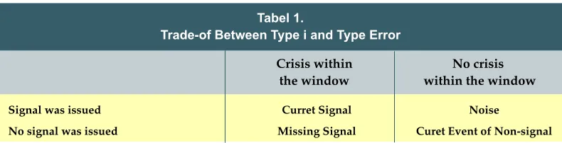
5. Type I and Type II Error in Early Warning System Models
There are two possible errors that can happen in an early warning system model, i.e.
not issuing any signal when currency crisis occurs in upcoming months (also called as type
I error), or giving signal when currency crisis does not occurs in upcoming months (noise or
type II error). From decision makers perspective, type I error causes bigger social loss than
type II error.
Tabel 1.
Trade-of Between Type i and Type Error
Signal was issued Curret Signal Noise
No signal was issued Missing Signal Curet Event of Non-signal
Crisis within No crisis
the window within the window
Basic set up for critical threshold of independent variable signals plays very important
role in determining whether type I or type II error will likely to occur. The lower the critical
threshold level, the higher probability of type II error occurrence. On contrary, the higher the
critical threshold level, the higher probability of type I error to occur.
Although the social loss caused by type II error is lower than by type I error, it does not
mean that the model should use the as-low-as-possible threshold level. The higher the
probability of type II error caused by lower level of critical threshold, the more inefficient the
early warning system. In this circumstance, the early warning system is no longer be able to
differentiate between normal and precrisis condition.
6. Previous Research Results
Findings from previous research are also taken as references for this study, where
individual leading indicator model; (2) Glick-Hutchison’s currency crisis and banking crisis
joint-models; (3) Bussiere-Fratzcher’s binomial and multinomial logit models; and (4)
Herrera-Garcia’s composite indicator model. Although this study does not use “discrete dependent
variable” model, Glick-Hutchison’s and Bussiere-Fratzcher’s findings are still interesting to
discuss as comparison to this study findings.
Before exposing findings from the four above mentioned studies, it is better to discuss
the definition of “currency crisis” used in each research. Kaminsky, Lizondo, and Reinhart
(1998) defined currency crisis as a condition where exchange market pressure (EMP) index
lies above EMPs’ mean plus three times of EMPs’ standard deviation. Glick and Hutchison
(2000) referred currency crisis as a movement of EMP (in their term: index of currency
pressure) above EMPs’ mean plus two times of EMPs’ standard deviation. Bussiere and
Fratzcher used the same threshold level of EMPs index as in Glick-Hutchison’s model to
define currency crises. Herrera and Garcia set mean plus 1.5 times standard deviation of
EMPs index (in their term: index of speculative pressure) as threshold level of currency
crises. In both definitions, higher EMP (in positive number) means higher tendency for a
currency to undergo devaluation or depreciation.
In Kaminsky-Lizondo-Reinhart’s and Glick-Hutchison’s model, EMP is defined as
weighted average value of nominal exchange rate and international reserves monthly
vola-tility, with higher weight is given to component with lower volatility. Meanwhile, Glick and
Hutchison, in their panel data model, defined index of currency pressure as weighted
aver-age of monthly real exchange rate and monthly percentage of reserve losses. The weights
are inversely related to variance of each component changes over the sample for each
country. By using real exchange rate, Glick and Hutchison expected that biases in currency
pressure measurement caused by ocassionally hyperinflation can be avoided.
In Herrera-Garcia’s model (1999), index of speculative pressure components
com-prises monthly percentage change of nominal exchange rate, interest rate, and
interna-tional reserves. These components are given the same weight, and normalized to have
zero mean (_=0) and unit variance (_=1).
Bussiere-Fratzcher’s model (2002) defines EMP as weighted average value of real
exchange rate montly volatility, monthly real interest rate change, and international reserves monthly volatility. Bussiere-Fratzcher model also gives higher weight to component with
lower volatility. The use of real term for exchange rate and interest rate volatility in
Bussiere-Fratzcher model is to deal with different inflation rates among countries selected as samples.
As their findings, Kaminsky-Lizondo-Reinhart found that several macroeconomic
vari-ables are working well as individual leading indicators of currency crisis. The indicators are
(1) national output (GDP); (2) exports; (3) real effective exchange rate; (4) stock index; and
(5) ratio of broad money to international reserves. These indicators issue at least one signal
24 months prior to a crisis.
Herrera and Garcia showed that the IMV worked well as a composite leading indicator in their 24-months-window early warning system models. Among the four different models
by its threshold setup technique, the “Simple Model” perform best in almost all of sample
countiers, except in Argentina and Brazil. The “Chartist Model” is the best model for Argen-tina, while the “DT Model” is best for Brazil. With regard to error types of signals issued ,
Herrera-Garcia study found higher numbers of type I error and lower numbers of type II
error in their models than in Kaminsky-Lizondo-Reinhart’s.
Bussiere and Fratzcher pointed out that their multinomial logit model (with three
cat-egories of dependent variable) could predict currency crisis probability more efficient than
ordinary binomial logit model. Variables that worked well in Bussire-Fratzcher study are: (1)
real exchange rate misallignment from its trend; (2) lending boom; (3) ratio of short term
debt to international reserves; (4) ratio of current account to GDP; (5) financial contagion;
and (6) economic growth. Bussiere and Fratzcher also found out that 20% was the optimum
threshold value for these variables to predict the probability of crisis. By applying the 20%
threshold level, they obtain 12 months as the optimum horizon (window) for their system.
Glick and Hutchison concluded that in general, banking crisis is a good indicator of
future currency crisis, but not the vice versa. Their other finding is that the simultaneous or almost simultaneous banking and currency crises (the twin crises) phenomenon are more
often to occur in developing and emerging countries than in developed countries. They also
found out that strong causality, joint-feedback relations between currency crises and
bank-ing crises only existed in financially-liberalized emergbank-ing countries.
Glick and Hutchison suggested further that monetary authority should take measures
to prevent banking crises, since it can reduce the possibility of currency crises occurrence.
On the other hand, currency crisis prevention measures (especially in emerging countries)
can also reduce the possibility of banking crisis occurrence. As long as central bank has
sufficient foreign reserves to defend the currency, Glick and Hutchison suggestion may
EMP RER RER
RER
res res
res r r
RER
i t i t i t
res
i t i t i t
r i t i t
work well. However, in extreme twin crises cases, where central bank suffers lack of foreign
reserves, “policy dilemma” becomes the rule. Pouring more liquid money to prevent
bank-ing system collapse will result in higher pressure for domestic currency to depreciate. On
contrary, defending the currency by raising interest rate will hurt commercial banks.
7. Models Specification
7.1 Currency Crisis Definition
Currency crisis definition in this study refers to Bussiere-Fratzcher’s definition. Due to
the single country nature of this study (not a panel data study), two modifications are made
to the original EMP equation in BussieFratzcher’s model. The first modification is to
re-place real exchange rate and interest rate with their nominal values, while the second is to
make new weighing method for EMP components.
Weighing method for the three components of EMP in this study is based on their
standard deviation. Higher weight is given to component with higher standard deviation,
based on consideration that variable with higher standard deviation generates stronger
pressure on exchange rate than the lower ones. The procedure of weighing is defined as
follows:
First, determine the ratio of weights among EMP components by using standard
de-viation of each component (ri; i = 1, 2, 3), Component with lowest standard deviation is set to be the benchmark category with the value of 1.
Second, determine the weight for each component by dividing each value of r1, r2, and r3 with total sum of r1, r2, and r3.
and where
r
1:
r
2:
r
3=
stdev X
(
1) :
stdev X
(
2) :
stdev X
(
3)
stdev X
(
1)
>
stdev X
(
2)
>
stdev X
(
3)
ϖ ϖ ϖ
1 2 31 2 3
:
:
=
r
:
:
R
r
R
r
R
r
3=
1
Meanwhile, currency crisis in this study is defined as any condition where EMP of an
observation is higher than EMPs’ mean plus one times EMPs’ standard deviation.
Cur-rency crisis definitions used by Kaminsky-Lizondo-Reinhart’s, Glick-Hutchison’s,
Herrera-Garcia’s, and Bussiere-Fratzcher’s models are not suitable for the case of Indonesia. These
definitions of currency crisis are unable to include the Rupiah’s 1986 devaluation, due to their very high threshold level of crisis
In mathematical term, currency crisis in this study is defined as:
R
=
r
1+
r
2+
r
3CC
if EMP
EMPs
SD EMPs
if others
t
=
>
+
1
0
(
)
7.2 Individual Leading Indicator Model Specification
Individual leading indicator model in this study uses a threshold level which will leave
20% best observations of a variable. Whenever an observation is higher than the threshold
level, a warning signal of currency crisis will be issued. Four below categories are used as
building blocks to construct ratios for indicators performance measurement:
1) Correct signal (labelled as “A”)
A correct signal is a signal that is followed by a currency crisis within 24 months period
after its issuance.
2) Type II error (labelled as “B”)
A type II error occurs when an indicator issue a signal, but not followed by any currency
crisis within the next 24 months period.
3) Type I error (labelled as “C”)
A type I error occurs when an indicator does not issue any signal within 24 months
period prior to an actual currency crisis.
4) Correct time when an indicator does not issue any signal (“D”)
When an observation shows that an indicator does not issue any signal and the absence
of signal is not followed by any currency crisis within the next 24 months period, the
Three following ratios are used to determine best indicators to be selected in
indi-vidual leading indicator model for early warning system7:
1) Percentage of Correctly Called Crises
Percentage of correctly called crises is measured as a ratio between numbers of
cor-rectly called crises to the number of actual currency crises. The higher this ratio, the
higher leading indicator’s ability to map actual currency crises occurrence. A good
indi-cator based on this criterion should at least issues one signal within the 24-months
window prior to the crises.In mathematical term, percentage of correctly called crisis is
expressed as follows:
2) Adjusted Noise to Signal Ratio
Adjusted noise to signal ratio is a measure of indicator’s efficiency in issuing warning
signals. Higher value of this ratio implies lower efficiency of an indicator in predicting
currency crises. As a rule of thumb, adjusted noise to signal ratio which is lower than or
equal to 100% shows that the respective indicator is still efficient. On contrary, an
indica-tor with higher than 100% adjusted noise to signal ratio is considered as not efficient. In
mathematical term, adjusted noise to signal ratio is expressed as:
3) Probability of Crisis Following a Signal Issuance
The third criterion used to determine best indicators is the probability of crisis following a
signal issuance. The higher the probability, the better an indicator performance will be. In
mathematical term, probability of crisis following a signal issuance is expressed as:
Percentage of correctly called crises
number of correctly called crises
number of actual crises
=
7 These criteria is taken from Kaminsky, Lizondo, and Reinhart (1998).
Adjusted noise to signal ratio
B B
D
A A
C
=
+
+
(
)
(
)
Probability of crisis following a signal issuance
A
(A
B)
=
+
In this study, to be considered as one among the bests, an individual leading
1) Be able to map at least 70% of all actual currency crises in Indonesia. It means the
indicator should issue at least one signal within 24 months period prior to an actual
crisis. In other words, the respective indicator should have equal to or higher than 70%
accuracy level.
2) Be efficient, which means that the adjusted noise to signal ratio should be lesser than or
equal to 100%.
3) Have greater than or equals to 50% probability of crisis occurrence following its signal
issuance.
7.3 Composite Leading Indicator Model Specification
Composite leading indicators in this study are constructed from best individual
lead-ing indicators. A composite indicator is made by summlead-ing up its standardized individual
indicator components. A signal will be issued by a composite indicator whenever an
ob-servation passes critical threshold level, a value that leaves only 20% highest obob-servations.
The three above mentioned criteria for individual indicators are also used to measure
com-posite leading indicators performance.
7.4 Research Procedures
The procedures of this research can be described as follows:
1) Identifying currency crisis occurrence, comprises:
a. Calculating monthly exchange rate volatilities, interest rate changes, and interna-tional reserves volatilities as components of EMPs
b. Measuring standard deviation of each EMPs component and creates ratios among the three standard deviations, with the lowest standard deviation set as the bench-mark and has the value of 1.
c. Summing up the ratios and divide each ratio to total sum as the weight for each component
d. Monthly EMP is measured by summing up all of its weighted components
e. Calculate EMPs’ mean and standard deviation for crisis critical threshold. The threshold is set as EMPs mean plus one of EMPs’ standard deviation.
2) Identifying signals from indicator, comprises:
a. Normalizing each observation of an indicator, by substracting an observation value from indicator’s mean, and dividing by indicator’s standard deviation
b. Sorting the normalized observation values, from the highest to the lowest
c. Selecting a threshold level that will leave 20% best observation of the respective indicator.
d. If any observation is greater than the critical threshold level, the indicator will issue a warning signal of currency crisis within upcoming 24-months.
3) Measuring indicator’s performance, comprises:
a. Comparing currency crisis and indicator’s warning signal issuance data for each vari-ables examined as candidates for leading indicators
b. A correctly called crisis is obtained by looking backward an indicator’s signal issuance data within 24-months period prior to a crisis, whether the indicator issue at least one signal or not. If the answer is yes, then the value of correctly called crisis equals to 1, otherwise 0. Numbers of correctly called crises is the sum of correctly called cases. Meanwhile, percentage of correctly called crises is calculated by dividing numbers of correctly called crisis to numbers of actual currency crises.
c. Correct signal (A), type II error (B), type I error (C), and correct event of no signal issuance (D) is obtained by looking forward currency crises data. If a crisis occurs within 24-months period following a signal issuance, then it should be “A”, otherwise “B”. If an indicator does not issue any signal, but at least one crisis does occur within the 24-months forward period, then it should be “C”, otherwise “D”.
d. From the previous step, “Adjusted Noise to Signal Ratio” and “Probability of Crisis Following a Signal Issuance” can be calculated.
4) Selecting Best Indicators
a. Selecting ten best indicators (or more) based on percentage of correctly called crises criterion.
b. Selecting ten best indicators based on adjusted noise to signal criterion.
c. Selecting ten best indicators based on probability of crisis following a signal issuance.
Exchange Market Pressure Currency Crises Threshold Level
1983 1986 1989 1992 1995 1998 2001
Feb Feb Feb Feb Feb Feb Feb
Persen
45
25
5
-15
7.5 Data Source and Software Used
Data range for this study is from January 1981 to December 2002, except for JCI
(from April 1983) and balance of payment items (from March 1981). The data are taken from
the IMF’s International Financial Statistics (IFS) and Bloomberg’s Economic Statistics (ECST).
Monthly data of GDP, current account and financial account surplus are obtained by linearly
interpolating their quarterly values. GDP data is in its index value, with 1996 is set as the
base year.
Matlab version 6.0. Release 12 and Microsoft Excel 2000 are software used to
con-struct early warning system in this study. The two software are not used complementary
(except in tabulation of results which is done in Excel), as the models in this study are
deliberately built by using each software separately. The Matlab program of early warning
system is built to provide ready-to-use tool for examining each indicator faster. The Matlab
version is more adjustable than the Excel version, since one can change the window and
threshold level of early warning system easier. However, the Excel program is still used as
the benchmark to control the Matlab program from making errors. Both programs use the
if-then logic arguments as their building bricks.
8. Results and Analysis
8.1 Actual Currency Crises Cases
As already explained previously, currency crisis in this study is defined as a condition
where EMP passes EMPs’ mean plus one times EMPs’ standard deviation. Based on this
definition, the EMPs’ threshold level for currency crisis occurrence is 4.9%. Any condition
where EMP passes its threshold level is considered as a currency crisis. The following
table illustrates Rupiah exchange market pressure movement from February 1983 to
December 2002.
The weighing for EMP components are set as: 0.4 for exchange rate volatility; 0.3 for
international reserves volatility; and 0.3 for money market interest rate monthly change.
Hence, total value of weights equals to 1.0. The highest weight was given to exchange rate
volatility as it has the greatest standard deviation among all EMP components. The actual
currency crises occurence in Indonesia, along with EMP and its components values are
depicted in the following table:
March1983 10,8% 0,3% 1,4%-33,8%
April 1983 10,2% 38,1% -3,0% 19,0%
September 1986 14,2% 27,0% 0,6% -7,0%
October 1986 6,7% 13,7% -0,3% -2,4%
August 1997 19,0% 11,2% 49,2% -4,7%
October 1997 7,9% 18,4% -12,3% -9,6%
December 1997 20,0% 40,6% -1,5% -8,2%
January 19984 4,0% 96,8% 16,5% 9,4%
May 1998 6,6% 24,5% -7,3% 7,6%
June 1998 16,8% 36,8% 1,1% -1,2%
January 1999 5,2% 12,4% 4,5% 4,6%
Table 2.
Actual Currency Crises in Indonesia and Their Exchange Market Pressures
Date of Crisis
Exchange Market Pressure
Exchange Rate Volatility (weight = 0.4)
Interest Rate Volatility (weight = 0.3)
International Reserves Volatility
(weight = 0.3)
EMPs historical data shows that eleven currency crises had occured in Indonesia
during February 1983 and December 2002. The March and April 1983 crises lead to “1983
Rupiah Devaluation”, as the government officially announced that the exchange rate was
changed to IDR 968.6 / USD, from previously IDR 699.1 / USD in February 1983. The
second devaluation within this period occured in October 1986, after Rupiah exchange
market pressure passed its threshold level in September and October 1986.
From all currency crises that had occured in Indonesia, the “1997-1999 currency
cri-ses series” was the severe. Opened with a crisis in August 1997, six other cricri-ses followed
in October 1997, December 1997, January 1998, May 1998, June 1998, and January
pressure reached 44.0% and Rupiah was dropped to IDR 9,662.5/USD from IDR 4,908.8/
USD in December 1997. The “1997-1999” crises series also had political consequences as
it became one among critical factors that forced Soeharto to resign from his presidency in
May 1998.
8.2 Models Examination Results 8.2.1 Individual Leading Indicators
Examination result of the 65 variables in this study shows that only few variables are
reliable as individual leading indicators for early warning system. In general, even more
limited numbers of indicators can satisfy all of the three criteria. For example, some
vari-ables can accurately map all of actual currency crises, but these varivari-ables are not efficient
by often issuing unnecessary signals. On contrary, other variables are very efficient, but
missed a lot numbers of actual crises.
Result of indicators examination by using the overall three criteria shows that only five
variables are eligible to be selected as core indicators in individual leading indicator model.
The indicators are: (1) Rupiah REER misalignment over its trend value; (2) foreign assets
growth in Domestic Money Banks; (3) financial account surplus; (4) M0 growth; and (5) ratio
of financial account surplus to GDP.
These indicators have higher than 70% percent accuracy in mapping actual currency
crises, high efficiency level (reflected by their adjusted noise to signal ratio, which are lower
than 100%), and high probability of currency crisis following a signal issuance (higher than
50%). Among the core individual leading indicators for early warning system, only “REER
misalignment over its trend” and “Deposit Money Banks foreign assets growth” can predict
all of actual currency crises occurence with 100% level of accuracy.
REER Misalignment over Trend 100,0% 11,7% 80,0%
DMBs Foreign Assets Growth 100,0% 30,0% 61,0%
Financial Account Surplus 90,9% 32,4% 59,2%
M0 Growth 72,7% 32,4% 59,2%
Financial Account Surplus / GDP 72,7% 41,7% 52,9%
Table 3.
Best Individual Leading Indicators in Overall Criteria
Indicator
Percentage of Correctly Called
Crises
Adjusted Noise Signal
Ratio
Probability of Crisis Following A
8.2.2 Composite Leading Indicators
The composite leading indicators in this study are made from combinations of the
overall-criteria five best individual leading indicators. A restriction is imposed so that
“finan-cial account surplus” variable will not meet “ratio of finan“finan-cial account surplus to GDP”
vari-able in the same combination. Overall, 18 possible combinations of composite indicators
can be made. From all of these combinations, 9 combinations are made of two elements, 7
combinations of three elements, and only 2 combinations of four elements. The restriction
causes combination made of five elements ineligible for composite indicators.
Examination results show that 17 out of 18 composite leading indicators can meet the
overall criteria. The only composite indicator with poor result is “XY”, a combination of
“fi-nancial account surplus” and “M0 growth” variables. The seventeen composite indicators
perform better than the five best individual leading indicator, mainly by their higher
effi-VW 100.0% 9.1% 83.7%
VWY 100.0% 11.7% 80.0%
VWZ 100.0% 13.8% 77.3%
VWYZ 100.0% 15.2% 75.6%
VZ 100.0% 17.6% 72.7%
VWX 100.0% 18.2% 72.1%
WZ 100.0% 26.1% 64.3%
VY 100.0% 26.4% 64.0%
VYZ 100.0% 32.4% 59.2%
WX 90.9% 17.6% 72.7%
YZ 90.9% 40.0% 54.0%
VWXY 81.8% 13.4% 77.8%
WXY 81.8% 20.5% 69.6%
VX 81.8% 21.0% 69.0%
WYZ 81.8% 24.2% 66.0%
VXY 81.8% 25.7% 64.6%
WY 81.8% 29.1% 61.7%
Table 4.
Best Composite Leading Indicators in Overall
Composite Indicator
Percentage of Correctly Called
Crises
Adjusted Noise Signal
Ratio
Probability of Crisis Following A
Signal Issuance
NOTE:
V REER Misalignment over Trend
W DMBs Foreign Assets Growth
X Financial Account Surplus
Y M0 Growth
ciency level and higher probability of crisis following a signal issuance. These composite
indicators can also map actual currency crises occurence with higher than 80% level of
accuracy, and even nine among them reach 100%.
The table shows that the nine best composite leading indicators contain either
“Ru-piah REER misalignment over its trend value” or “Deposit Money Banks’ foreign assets
growth” variables as its element.
8.3 Analysis
As already shown previously, “Rupiah REER misalignment over its trend value”,
“De-posit Money Banks’ foreign assets growth”, “financial account surplus”, “base money growth”,
and “ratio of financial account surplus to GDP” are best individual leading indicators. From
these individual indicators, 17 best composite leading indicators can also be constructed.
The following part is a thorough analysis about the nature and behaviour of the these
indi-vidual indicators with regard to Indonesian economy historical data.
8.3.1 REER Misalignment over Its Trend Value
“Rupiah REER misalignment over its trend value” is the best of the best individual
leading indicators. Combined with “Deposit Money Banks’ foreign assets growth” variable,
this variable produce “VW” composite indicator, which is the best among all composite
indicators. Rupiah REER movement along with its quadratic trend and misalignment since
January 1981 until December 2002 are depicted in the following graph:
Persen
Rupiah REER Rupiah REER Trend Line 0
50 100 150 200 250
1981 1984 1987 1990 1993 1996 1999 2002
Jan Jan Jan Jan Jan Jan Jan Jan
Graph 3. Real Effective
Excellent performance of “Rupiah misalignment over its trend value” as a leading
indicator of currency crises can be seen from its historical data. Prior to devaluation against
US Dollar in April 1983 and September 1986, Rupiah was overvalued against its trend.
Before the great crises series started in August 1997, Rupiah was also overvalued against
its trend, and even reached the highest level of misalignment in April 1997 at 28.23%.
Based on theory, real overvaluation of a currency against its trend is one among
possible causes of currency crisis. Real overvaluation leads to trade balance deterioration,
hence reduces foreign reserves accrued from international trade. The condition depletes
foreign reserves owned by central bank, and weaken central bank’s ability to defend
cur-rent exchange rate level when attacks toward domestic currency take place. To examine
trade balance deterioration, it is better to use trade balance surplus growth rather than trade balance surplus itself, as the previous is a flow variable.
Although trade balance surplus growth is not a good individual leading indicator in
this study, due to its lower than 50% probability of crisis following a signal issuance,
histori-cal data of this variable supports the claim that currency real overvaluation did happened
prior to all currency crises occurrence in Indonesia. Prior to the onset of 1997 – 1999
currency crises series, Indonesia suffered trade balance deterioration in all months of 1995
and several times in 1996 and 1997, as reflected in its negative values of trade balance
surplus growth.
As shown in the following picture, to obtain 20% best observation of “Rupiah REER
misalignment over its trend value” variable, 15.1% is selected as the threshold level. Any
Persen
0%
-300 -50 200 450 700
1995 1996 1997 1998 1999
Jan Sep Mei Jan Sep Mei Jan Sep
Graph 4. Indonesia’s
Rupiah REER misalignment over its trend that is greater than 15.1% will produce a warning
signal of currency crisis.
Rupiah's REER Misalignment over Its Trend Threshold Level
5,11%
-60 -20 20 60
1981 1984 1987 1990 1993 1996 1999 2002
Jan Jan Jan Jan Jan Jan Jan Jan
Persen
Graph 5. Rupiah REER Misalignment over Its Trend Value
“Rupiah REER misalignment over its trend value” indicator can issue a signal as early
as 24 months prior to a crisis, as in September 1997 crisis. In average, “Rupiah REER
misalignment over its trend value” indicator can issue a warning signal at least in 21 months
prior to a currency crisis. However, the indicator does not consistently issue warning signals
in every months within the window, as in 1983 and 1986 Rupiah devaluation cases. It only
issues nine warning signals prior to April 1983 devaluation, and seven signals prior to
Octo-ber 1986 devaluation.
8.3.2 Deposit Money Banks’ Foreign Assets Growth
Deposit Money Banks’ foreign assets are loans in foreign currency lent by Deposit
Money Banks to the debtors. These loans are used by borrowers to meet their payment
obligations in foreign currencies, such as for exports and imports financing. Some exports –
imports activities require exporters and importers to prepay the costs of warehousing,
ship-ments, and insurances prior to the acceptance of payments or goods.
Although foreign assets are one source of revenues for banks, they also contain risks.
Foreign assets, especially unhedged ones, are very vulnerable to foreign exchange
expo-sures. If the debtors earn their revenues in domestic currency, unanticipated exchange rate
turbulences may cause them to default their obligations. This condition will result in banking
Deposit Money Banks' Foreign Assets Growth
Threshold Level
18.0% Persen
-50 -15 20 55 90
1981 1984 1987 1990 1993 1996 1999 2002
Jan Jan Jan Jan Jan Jan Jan Jan
awared as it becomes an indication of increasing banking system fragility and vulnerablity
toward exchange rate exposures.
It is interesting to note that all of currency crises in Indonesia were preceded by or
occured at the same time with the banking crises. In a condition where currency and banking
system crises occur in the same time, central bank will hesitate to increase interest rate to
defend its exchange rate target level. An interest rate increase will hurt the banking system,
as Deposit Money Banks have to pay higher deposits interest and face greater risks of
obligors default. Hence, although foreign assets growth in Deposit Money Banks was not
the trigger of a currency crises occurrence, it did worsen the crises.
In testing “Deposit Money Banks’ (DMBs) foreign assets growth” performance as a
leading indicator, the variable is expressed in million US Dollar. This treatment is made in
order to avoid bias caused by exchange rate turbulance. If the variable is expressed in
Rupiah, foreign assets growth will rocket during the crisis period, while the real value
expressed in US Dollar grow more moderately.
Based on examination results, “DMBs foreign assets growth” is in the second place
among all best individual leading indicators. Together with “Rupiah REER misalignment
over its trend value”, this variable construct “VW”, the best composite leading indicator.
From its historical trend, “DMBs foreign assets growth” indicator issued at least one
signal prior to all currency crises occured in Indonesia. The threshold level for a signal
issuance of “DMBs foreign assets growth” is 18.0%. “DMBs foreign assets growth” indicator
was able to issue a warning signal as early as 24 months prior to 1983 and 1986 Rupiah
devaluations.
In average, “DMBs foreign assets growth” indicator can issue at least a warning signal
in 21 months prior to a currency crisis. Nevertheless, “DMB foreign assets growth” indicator
did not consistently issuing signals in every months within the 24-months window. Prior to
the onset of currency crises series in August 1997, the earliest signal was issued in November
1995. The signals became more frequent within seven-months prior to August 1997.
8.3.3 Financial Account Surplus
“Financial account surplus” is the third best individual leading indicator. Combined
with “Rupiah REER misalignment over its trend value” an