Vol. 10, 2016-25 | October 19, 2016 | http://dx.doi.org/10.5018/economics-ejournal.ja.2016-25
Does Uncertainty Affect Non-response to the
European Central Bank’s Survey of Professional
Forecasters?
Víctor López-Pérez
Abstract
This paper explores how changes in macroeconomic uncertainty have affected the decision to reply to the European Central Bank’s Survey of Professional Forecasters (ECB’s SPF). The results suggest that higher (lower) aggregate uncertainty increases (reduces) non-response to the survey. This effect is statistically and economically significant. Therefore, the assumption that individual ECB’s SPF data are missing at random may not be appropriate. Moreover, the forecasters that perceive more individual uncertainty seem to have a lower likelihood of replying to the survey. Consequently, measures of uncertainty computed from individual ECB’s SPF data could be biased downwards.
(Published in Special Issue Recent Developments in Applied Economics)
JEL D81 D84 E66
Keywords Non-response; uncertainty; Survey of Professional Forecasters; European Central Bank
Authors
Víctor López-Pérez, Department of Economics, Technical University of Cartagena, Cartagena, Spain, [email protected]
Citation Víctor López-Pérez (2016). Does Uncertainty Affect Non-response to the European Central Bank’s
Survey of Professional Forecasters? Economics: The Open-Access, Open-Assessment E-Journal, 10 (2016-25): 1—
1
Introduction
The European Central Bank’s Survey of Professional Forecasters (ECB’s SPF) is gaining prominence in recent years not only for policy analysis (ECB 2014a, 2014c) but also for research (Lyziak and Paloviita 2016; Glas and Hartmann 2016; Kenny and Melo Fernandes 2016; Poncela and Senra 2016; Abel et al. 2015; Bowles et al. 2010; Conflitti 2011; Kenny et al. 2012). The SPF was launched in the first quarter of 1999 and collects expectations of inflation, GDP growth and the unemployment rate in the euro area for different forecast horizons. These expectations are submitted quarterly by professional forecasters located in the European Union.
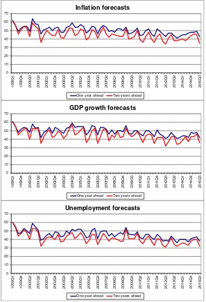
The number of forecasts collected by the ECB varies from one quarter to the next. Figure 1 shows the number of participants that submitted a point forecast of a variable of interest (inflation, GDP growth or unemployment) for selected forecast horizons (one and two years ahead) in each survey round.1 Figure 2 shows the same statistics for density forecasts. The number of replies is not constant over time because some participants skip some survey rounds, for instance due to holidays.2 Moreover, some of the respondents to the first waves of the SPF stopped replying in later rounds, a feature of panel surveys commonly known as
attrition (Den Van Berg et al. 1994).3
Despite the growing interest in the SPF, there is a surprisingly scarce amount of research on the factors that affect non-response to this survey. Engelberg et al. (2011) and López-Pérez (2016) explored the effects of changes in the composition of the panel of participants on aggregate results from the survey, but the decision to reply is not investigated. Furthermore, Engelberg et al. (2011: 1076) concluded that,
_________________________
1 The SPF collects two types of forecasts. A pointforecast is a scalar (e.g. “inflation in 2015 is
ex-pected to be 0.7%”). A density forecast is a vector of subjective probabilities over a set of predefined intervals (e.g. “there is a 60% probability that inflation in 2015 will be between 0.5% and 0.9% and 40% probability that it will be between 1.0% and 1.4%”).
2 There is a clear seasonal pattern in the number of replies: the ECB systematically receives the lowest number of forecasts in Q3 surveys, which are conducted in the second half of July.
3 In this context, attrition is defined as the gradual reduction over time in the number of participants
Figure 1: Number of participants that submitted point forecasts in each survey round
One year ahead Two years ahead
0
One year ahead Two years ahead
0
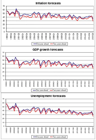
Figure 2: Number of participants that submitted density forecasts in each survey round
One year ahead Two years ahead
0
One year ahead Two years ahead
0
“We observed in the Introduction that, in the absence of knowledge of the forecaster recruitment and participation process, the assumption that data are missing completely at random is not refutable. Hence one might argue that this simplifying assumption should be maintained until evidence to the contrary emerges. To forestall endless debate about the validity of this or other simplifying assumptions, we see a strong need for research that sheds light on the forecaster recruitment and participation process. Only then will it become possible to reach consensus on the seriousness of the composition issue in survey response.”
This paper is, to the best of my knowledge, the first attempt to investigate the determinants of response to the ECB’s SPF. In particular, it analyses the effects of macroeconomic uncertainty on the probability that panellists reply to the survey. Theoretically, more uncertainty about the economic environment could make the production of macroeconomic forecasts more difficult and costly. For example, updating the forecasting models in a more uncertain environment, like in the turning points of the business cycle, may require more time and effort than in calmer periods because the empirical relationships could suffer from structural breaks, some explanatory variables may become less relevant than before and new variables could become more important, like financial variables after the start of the financial crisis in 2007. These higher production costs of the forecasts at uncertain times could lower the incentives to participate in the SPF, especially the incentives to submit density forecasts because most SPF forecasters do not use them for purposes other than the SPF (79% of them, according to ECB 2014b). Moreover, forecasters who are not confident enough about their outdated forecasting models may decide not to respond to the survey until their models are updated. I label this hypothesis of a negative relationship between uncertainty and response to the survey as the production-cost hypothesis.
Anecdotal evidence supporting this hypothesis relates to the announcement made by the Deutsche Institut für Wirtschaftsforschung (DIW), which in 2009 said that it would not publish forecasts for the German economy for 2010 because there was too much uncertainty after the financial crisis started.4
_________________________
Another possible channel from uncertainty to response to the ECB’s SPF is related to the strategic behaviour by professional forecasters.5 If they believe that their forecasts may have an effect on the monetary-policy actions by the ECB they may have more incentives to reply at uncertain times: when less is known about the state of the economy, policy-makers could put more weight on the information provided by professional forecasters. I label this hypothesis of a positive relationship between uncertainty and response to the survey as the strategic-behaviour hypothesis.
Preliminary evidence of the link between uncertainty and response can already be found in Figures 1 and 2. It is typically assumed in forecasting that uncertainty increases with the forecast horizon. If this is true, and if uncertainty reduces the incentives to reply (the production-cost hypothesis), the number of forecasts submitted by SPF panellists for each macroeconomic variable should decline with the forecast horizon. And this is what is found in the data: the number of two-year-ahead forecasts in Figures 1 and 2 is consistently below the number of one-year-ahead forecasts.
More preliminary evidence on the relationship between uncertainty and response is obtained from the change in response rates across survey rounds within the calendar year for two forecast horizons, one whose length is always the same (e.g. forecasts two years ahead) and another whose length is shrinking over the course of the year (e.g. forecasts for the next calendar year). If uncertainty declines with the forecast horizon and less uncertainty encourages more replies, the response rates for forecasts with a shrinking horizon length should increase by more (or decrease by less) than the response rates for forecasts with a fixed horizon. Figure 3 shows the average change (in percentage points) in the response rate in Q2, Q3 and Q4 surveys compared to the previous survey for density forecasts two years ahead and density forecasts for the next calendar year. For all variables surveyed, the response rates for the forecasts with a shrinking horizon length rose more (or fell less) than the response rates for the forecasts with a fixed horizon length. This behaviour is consistent with a negative relationship between uncertainty and the likelihood of replying.
_________________________
Figure 3: Average changes in the response rate for selected density forecasts in Q2, Q3 and Q4 survey rounds with respect to the previous round
0.4
Next calendar year Two years ahead
0.4
Next calendar year Two years ahead
0.2
The finding of significant effects from macroeconomic uncertainty on SPF response may have implications for policy analysis based on SPF data. First, if fewer responses are received when uncertainty surges, the information content of the survey may be eroded during periods of heightened uncertainty, precisely when the information from the survey may be needed the most.
And second, a negative correlation between response and uncertainty could make SPF-based estimates of uncertainty biased downwards. If forecasters perceiving more uncertainty are less likely to reply, the estimates of uncertainty based on the data submitted by the responding panellists may underestimate the overall degree of uncertainty perceived by SPF panellists.
This paper estimates a model of the probability of response to the SPF as a function of uncertainty with individual response data. The estimation results are presented in Section 3. Section 4 explores the relationship between individual GDP growth forecasts and measures of subjective uncertainty, controlling for sample selection. If panellists perceiving more uncertainty are less likely to reply, the negative effect of uncertainty on expected GDP growth may be overstated when sample selection is not taken into account. Section 5 concludes and outlines directions for future research.
2
The data
Most of the data used in this paper is obtained from the ECB’s SPF. 103 forecasters have replied at least once to the survey, although average participation is around 60 forecasters per round. The panel is unbalanced, as many forecasters sometimes do not reply while others have left the panel and have been replaced with new panellists. The identity of the participant who submitted each forecast is kept confidential but the ECB’s SPF website indicates that professional forecasters “are experts affiliated with financial or non-financial institutions based within the European Union”. Non-financial institutions include labour and business organisations, research institutes and universities.
for each variable.6 The forecast horizons used in this paper are rolling horizons one and two years ahead.7 Therefore, the SPF provides data on the subjective probabilities that individual forecasters assigned to different macroeconomic events. For instance, the data from the ECB’s SPF webpage indicates that, in October 2013, forecaster number 1 assigned 70% probability to the September 2014 inflation rate in the euro area being between 1.5% and 1.9%.
Response data is constructed from the raw survey data available on the ECB’s SPF website. The sample period is 1999 Q1–2015 Q3. Time series of a number of dummy variables are created. These dummies take the value 0 when forecaster i
did not submit a forecast of variable j for forecast horizon h in survey round t, and take the value 1 otherwise. Therefore, each forecaster’s response is characterised by 12 dummy variables: three variables of interest (inflation, GDP growth and unemployment) times two types of forecasts (point and density forecasts) times two forecast horizons (one and two years ahead).
Out of 116 forecaster identification numbers included in the SPF dataset, 13 never submitted a forecast to the ECB. These forecasters were removed from the sample.8 Moreover, not all forecasters received invitations to participate in the SPF in 1999 Q1 but many of them were invited later on. The survey round when each forecaster was first invited to participate is unknown. It is assumed that a participant was first invited to participate in round X if his/her longest period without submitting any forecast to the ECB was from 1999 Q1 to survey round X. 29 forecasters are in this situation, and their “zeros” before the assumed invitation date are treated as missing data in their dummy variables of response.9
_________________________
6 Details on the intervals available to SPF forecasters, including their changes over time, and on the forecast horizons surveyed in each SPF round can be obtained from the document “ECB Survey of Professional Forecasters (SPF): description of SPF dataset”, available here:
http://www.ecb.europa.eu/stats/prices/indic/forecast/shared/files/dataset_documentation_csv.pdf??8b 0b9ba730b2241d43fec92dacd2944d.
7 Other forecast horizons available in the SPF are the current calendar year, the next calendar year, the calendar year after the next and five calendar years ahead.
8 Forecaster identification numbers 12, 21, 25, 27, 51, 69, 74, 75, 77, 78, 79, 81 and 83.
9 Forecaster identification numbers 8 (first reply: 2007 Q2), 15 (2000 Q1), 22 (2000 Q2),30 (1999
Q4), 41 (1999 Q2),58 (2006 Q4), 80 (2001 Q2),84 (2001 Q2),96 (2000 Q2),97 (2004 Q1),98
Furthermore, the panel of participants is subject to attrition, with the number of participating panellists gradually declining over time. Attrition in the context of the SPF may occur, among other reasons, because the forecaster becomes bored with the ECB’s SPF, the forecaster leaves the participating institution and the contact details are not updated, the participating institution disappears, or the participating institution merges with another participating institution. Attrition results in the absence of replies by some panellists from a particular date until the end of the sample. It is assumed that a participant left the panel immediately after round Y-1 if his/her longest period without submitting any forecast to the ECB was from survey round Y to 2015 Q3.10 30 forecasters meet this condition and their “zeros” after their last reply are treated as missing data in their dummy variables of response.11,12
Turning now to the measure of uncertainty, the data is obtained from López-Pérez (2016) where several measures of individual uncertainty are computed from SPF density forecasts. One of these measures, the Gini index of the individual density forecast, is used in this paper.13
Borrowed from the literature on income and wealth inequality, the Gini index (Gini 1955) is based on the Lorenz curve (Lorenz 1905). This curve is typically used to represent how much wealth is in the hands of the poorest x% of the
_________________________
Q2),105 (2008 Q2),106 (2009 Q3), 107 (2008 Q2),108 (2008 Q2),109 (2010 Q2),110 (2010 Q4),
111 (2011 Q3),112 (2011 Q3),113 (2011 Q4), 114 (2014 Q3), 115 (2014 Q3) and 116 (2015 Q2).
10 This condition is checked after removing the non-response period at the beginning of the sample for the panellists whose identification numbers appear in footnote 9.
11 Forecaster identification numbers 9 (last reply: 2007 Q4), 10 (2010 Q3), 11 (2010 Q1), 13 (2000
Q1), 17 (2006 Q2), 18 (2010 Q1), 19 (2011 Q4),28 (2010 Q4),33 (2013 Q1),34 (2001 Q1),40
(2009 Q4),43 (2000 Q3), 44 (2000 Q2),46 (2001 Q2),50 (2009 Q4),53 (2004 Q1),55 (2001 Q1),
56 (2014 Q2),60 (2009 Q2), 62 (2007 Q2), 64 (2002 Q4),66 (2004 Q3),71 (2004 Q3),73 (2011
Q3),76 (2008 Q3),86 (1999 Q1),87 (2003 Q3),100 (2009 Q1),106 (2013 Q2) and109 (2012 Q2).
12 Attrition may also be the outcome of a deliberate decision by a participating institution to discontinue its contribution to the survey because of cost-benefit considerations. If increases in uncertainty augment the cost of forecasting, the removal of these observations would bias the results
presented in this paper against any negative effect of uncertainty on response.
population. The Lorenz curve may also be applied to the analysis of uncertainty with SPF data by representing the cumulative probability allocated to the x% less likely intervals of a density forecast.
If a forecaster faces no uncertainty, her density forecast would have probability one in just one interval. In this case, the Lorenz curve would be zero from the first interval to the one before the last and then it would jump to 1 in the last interval. On the contrary, if a forecaster faces maximum uncertainty, her density forecast would have the same probability allocated to every interval. Then, the Lorenz curve would increase uniformly from the first interval to the last.
The individual Gini index of uncertainty is defined as the distance between the Lorenz curve under maximum uncertainty and the Lorenz curve of the individual density forecast divided by the area below the Lorenz curve under maximum uncertainty:
∑
∑
= =
− −
= n
i i n
i
i i
x lc x G
1 1
) (
(1)
where n is the number of intervals, x is the nx1 vector (1/n, 2/n,…, 1)’, and lc is the nx1 vector of ordinates from the Lorenz curve of the individual density forecast. As the original Gini index declines with uncertainty, the sign was changed to turn it into an index that increases with uncertainty.14
The Gini index has two advantages over the most frequently used measure of uncertainty based on density forecasts, the standard deviation of the individual density forecast. First, the Gini index takes its maximum value when the density forecast is uniform, i.e. when the forecaster faces maximum uncertainty and all the intervals look equally likely. Note that the standard deviation of a density forecast reaches its maximum when the forecaster puts 0.5 probability in the lowest interval and the other 0.5 in the highest interval. Obviously, the formulation of the latter density forecast requires a lot of information, e.g. that the probability of an
_________________________
14 This formula is the discrete approximation to the area between the Lorenz curve under maximum
uncertainty and the Lorenz curve of the density forecast. If n were infinity, G would be bounded
between -1 and 0. As n in the ECB’s SPF is large but not infinity, the Gini indices of uncertainty
outcome located in the middle intervals is zero. This amount of information is completely at odds with the notion of maximum uncertainty.
The second advantage of the Gini index over the standard deviation of a density forecast is that a statistician that wants to compute the standard deviation needs to make an assumption on how probabilities are distributed within each interval. López-Perez (2016) shows how different assumptions may lead to different time series of aggregate macroeconomic uncertainty in the euro area. The Gini index does not require this assumption.
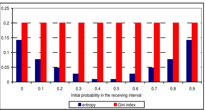
An alternative measure of uncertainty that can be computed from a density forecast is the entropy. As the Gini index, the entropy takes its maximum value when the density forecast is uniform and it does not need any assumption regarding the distribution of the probabilities within each interval. However, the Gini index has an advantage over the entropy: the non-linear nature of the entropy implies that the effect on the entropy from a certain change in the probabilities of a density forecast depends on the initial values of these probabilities. In the context of a simple example with two possible outcomes, Figure 4 shows that moving 0.1 probability from one outcome to the other leads to larger absolute changes in the entropy when the probabilities of the two outcomes are very different, i.e. when the level of entropy is smaller. The Gini index does not suffer from this drawback.15
This property of the entropy is relevant in the context of the ECB’s SPF because some forecasters assign zero probability to too many intervals. This behaviour has been labelled “overconfidence” and worsens forecasting performance (Kenny et al. 2015). The entropy of the density forecasts submitted by overconfident forecasters is smaller than the entropy of the density forecasts submitted by more “prudent”, better-performing forecasters. As changes in the entropy are larger when the initial level of entropy is smaller, changes in the average entropy would be relatively more affected by changes in the behaviour of the overconfident forecasters, whose forecasting performance, again, is worse. It is like putting more weight on the worst forecasters for the calculation of the aggregate measure of uncertainty.
_________________________
Figure 4: Illustration of the absolute changes in the entropy and the Gini index when 0.1 probability is moved across intervals (example with two intervals)
For these reasons, I prefer to use the Gini index to measure individual uncertainty. The aggregation (averaging) of the individual Gini indices across the SPF panellists that replied to two consecutive survey rounds allows for the calculation of a quarterly measure of percentagechanges in uncertainty from one survey round to the next. Using data from the panellists that replied to two consecutive rounds avoids mixing the concept of interest, that is, the changes in uncertainty perceived by a group of forecasters that remains fixed during two consecutive survey rounds, with a distortion in the estimates of aggregate uncertainty generated by the fact that some forecasters only replied once during these two rounds.16
Compounding the quarterly changes in uncertainty from one round to the next, a series representing the percentage change in the aggregate Gini index of uncertainty since 1999 Q1 is obtained for each macroeconomic variable and
_________________________
16 These percentage changes are shown on Figure 4 in López-Pérez (2016). The interested reader may find all the details about the construction of the aggregate Gini indices of uncertainty in that paper.
0 0.05 0.1 0.15 0.2 0.25
0 0.1 0.2 0.3 0.4 0.5 0.6 0.7 0.8 0.9
Initial probability in the receiving interval
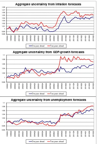
forecast horizon (Figure 5).17 For instance, aggregate uncertainty computed from the density forecasts of GDP growth two years ahead has been around 8% higher since the start of the financial crisis compared to its level in 1999 Q1, around 4% higher than in the previous peak in 2003 Q4, and around 6% higher than just before the financial crisis.
These aggregate-uncertainty measures show an increase in uncertainty during the period between 2000 and 2002, followed by a mild decline from 2003 to 2008. A jump in uncertainty occurred around the start of the financial crisis, after which uncertainty has remained relatively stable (the exception being the uncertainty measures computed from unemployment forecasts, which have kept on rising).
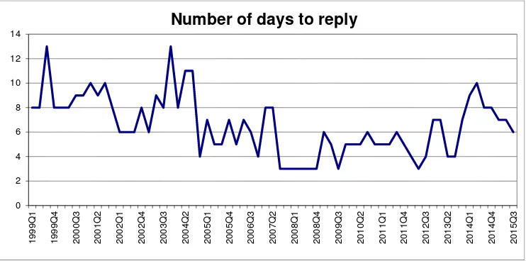
In order to achieve the goal of better understanding the relationship between uncertainty and response, the effects on the probability to reply from other variables need to be taken into account. In other words, there is a need to control for other variables to isolate the effect of uncertainty on response. In particular, for any given level of uncertainty, the probability of response is expected to be higher when respondents have more time to fill in the questionnaire. Therefore, a control variable will be used in the empirical exercise, namely, the number of days given to SPF panellists by the ECB to submit their forecasts during each survey round. This variable can be found in the document “Dates when the SPF has been conducted and published” downloaded from the ECB’s SPF webpage.18 Figure 6 shows the number of days given to SPF participants to submit their forecasts during each survey round.
_________________________
17 To be precise, if cjr is the percentage change of the average Gini index for variable j from round r
-1 to round r, its cumulative percentage change since 1999 Q1, ccjr, would be:
∑
The results of this paper are obtained with the approximation shown on the right side of the equation, as the approximation error is tiny.
18 The link to the document is:
Figure 5: Measures of aggregate uncertainty by variable and forecast horizon (Gini index
Aggregate uncertainty from inflation forecasts
One year ahead Two years ahead
0.98
Aggregate uncertainty from GDP-growth forecasts
One year ahead Two years ahead
0.96
Aggregate uncertainty from unemployment forecasts
Figure 6: Number of days given to SPF panellists to submit their forecasts to the ECB during each survey round
3
The effect of uncertainty on response to the ECB’s SPF
This section explores the effects of macroeconomic uncertainty on response to the ECB’s SPF. Let’s start with a non-parametric approach, calculating the partial Kendall’s tau rank correlation coefficient between the seasonally-adjusted response rates to the survey and aggregate uncertainty (Kendall 1938).19 This coefficient measures the co-movement in the ranks between two variables after removing the effect of a third variable, in this case the number of days to reply. It varies between –1 (perfectly negative rank correlation) to +1 (perfectly positive rank correlation), with a value of 0 indicating no rank correlation.
Table 1a shows the partial Kendall’s tau-b coefficient, which controls for ties in the rankings, between aggregate uncertainty and response rates. The first
_________________________
19 The response rate is defined as the number of responses divided by the number of non-attritioned forecasters invited to participate. Its seasonal component has been removed using TRAMO-SEATS (Gómez and Maravall 2001). The seasonal component of aggregate uncertainty is not removed because it is tiny.
Table 1: Partial Kendall’s tau-b rank correlation coefficients
a) Rank correlation between the response rate for different forecasts surveyed in the ECB’s SPF and different measures of aggregate uncertainty:
Forecasted variable
Aggregate uncertainty measure Gini one year ahead
Point forecasts –0.38 –0.19 –0.34
Density forecasts –0.49 –0.16 –0.31
Inflation two years ahead
Point forecasts –0.50 –0.27 –0.36
Density forecasts –0.54 –0.29 –0.37
GDP growth one year ahead
Point forecasts –0.32 –0.16 –0.31
Density forecasts –0.42 –0.19 –0.42
GDP growth two years ahead
Point forecasts –0.44 –0.18 –0.25
Density forecasts –0.51 –0.12 –0.25
Unemployment one year ahead
Point forecasts –0.49 –0.08 –0.25
Density forecasts –0.54 –0.06 –0.24
Unemployment two years ahead
Point forecasts –0.36 –0.12 –0.20
Density forecasts –0.43 –0.14 –0.26
b) Rank correlation between the response rate for different forecasts surveyed in the ECB’s SPF and the number of days to reply:
Forecasted variable
Aggregate uncertainty measure Gini one year ahead
Point forecasts 0.24 0.23 0.32
Density forecasts 0.36 0.34 0.45
Inflation two years ahead
Point forecasts 0.20 0.26 0.36
Density forecasts 0.18 0.24 0.34
GDP growth one year ahead
Point forecasts 0.18 0.21 0.31
Density forecasts 0.17 0.21 0.38
GDP growth two years ahead
Point forecasts 0.17 0.24 0.35
Density forecasts 0.22 0.30 0.49
Unemployment one year ahead
Point forecasts 0.21 0.19 0.32
Density forecasts 0.32 0.28 0.46
Unemployment two years ahead
Point forecasts 0.25 0.23 0.34
column uses the Gini index to measure uncertainty as explained in Section 2. The partial rank correlation is negative, ranging from –0.32 to –0.54. It suggests that increases in aggregate uncertainty are accompanied with declines in response rates. This result is consistent with the production-cost hypothesis: the incentives to reply to the survey decline with uncertainty because the cost of producing the forecasts is higher.
The second column in Table 1a uses the standardised 12-month and 24-month VSTOXX indices of stock market volatility (the European VIX index) as proxies for macroeconomic uncertainty instead of the Gini index.20,21
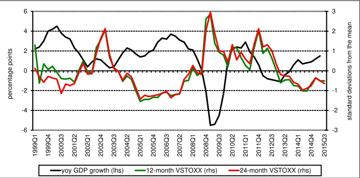
The rank correlation becomes weaker but this is mainly driven by the behaviour of the VSTOXX in the last three years of the sample: the non-conventional policy responses to the crisis by the central banks successfully calmed financial markets and reduced their volatility, but were less successful in reducing macroeconomic uncertainty (Bekaert et al. 2013). Figure 7 shows how the VSTOXX declines abruptly in 2012, just after the start of the ECB’s Long-Term Refinancing Operations (LTROs). That was also the year when Mario Draghi vowed to do “whatever it takes” to protect the euro. As a consequence, the VSTOXX has remained below its sample average since 2013 Q1, a period of significant macroeconomic uncertainty in the euro area due to the sovereign debt crisis.
This is a clear indication that VSTOXX indices may have become bad proxies for macroeconomic uncertainty during the last few years of the sample period. The third column in Table 1a shows the partial Kendall’s tau-b coefficient between response rates and the VSTOXX indices from 1999 Q2 to 2012 Q2. As expected,
_________________________
20 The VSTOXX indices are based on Eurostoxx 50 real-time options prices and are designed to reflect the market expectations of short-term and long-term volatility by measuring the square root of the implied variance across all options of a given time to expiration. The data is obtained from http://www.stoxx.com/download/historical_values/h_vstoxx.txt and is available since 1 January 1999. Quarterly data is computed by averaging daily data over the 90 days preceding the day when the ECB sent the SPF questionnaires to survey participants. The 1999 Q1 data point is excluded because it was the average of daily data for 30 days only.
21 Other measures of macroeconomic uncertainty have been developed in the literature but the two measures used in the paper, the Gini index from the SPF and the VSTOXX, have been selected
because they capture the degree of uncertainty perceived ex-ante by professional forecasters and
Figure 7: Year-on-year GDP growth rate in the euro area and standardised 12-month and 24-month VSTOXX indices
the coefficients become more negative than in the full sample. Table 1b confirms that an increase in the number of days to reply to the survey is accompanied by increases in the response rates.
An alternative approach to investigate the relationship between response rates and uncertainty is to regress the aggregate response rate to the survey for each variable and forecast horizon on the aggregate Gini index of macroeconomic uncertainty and the number of days to reply to the survey. The results of this analysis suggest that there is a cointegration relationship between response rates and macroeconomic uncertainty for all surveyed variables but the unemployment rate two years ahead.22 As expected, the long-run relationship is negative: when uncertainty increases the response rate falls. Moreover, the adjustment of response rates to deviations from the cointegration relationship is quite fast: between 37% and 79% of these deviations are absorbed after just one survey round.
_________________________
22 Results not shown here to save space. The interested reader may check these results in the working-paper version of this article available in the ECB website:
https://www.ecb.europa.eu/pub/pdf/scpwps/ecbwp1807.en.pdf?a491f34fcecfa3ca63adc274daeb0f01
3.1
Is response to the ECB’s SPF random?
Figures 1 and 2 showed that response to the ECB’s SPF has a strong seasonality component, with fewer responses in the survey rounds conducted in July each year. Furthermore, the number of replies are likely to increase with the number of days to reply, as forecasters have more time to prepare and submit their forecasts to the ECB. The missing-at-random assumption mentioned by Engelberg et al. (2011: 1076) suggests that response to the SPF should be a random process once the effects from seasonality and the number of days to reply are controlled for.
The missing-at-random assumption may be tested using a probit model of the conditional probability of response. If the assumption is correct, no variables other than the seasonal effect and the number of days to reply should be statistically significant in the estimated model. As this paper explores the effect of uncertainty on response, a measure of uncertainty is added to the model to test the missing-at-random assumption.
More precisely, the probability of replying by an individual forecaster may be modelled as follows:
( t t t U t D t i it)
it Q Q Q U D u
P =1)=Φβ+β1 1 +β2 2 +β4 4 +β +β + +ε
(
Pr (2)
where Pit is the dummy variable of response by panellist i in survey round t and
may take a value of zero or one; Qxt is a quarterly dummy variable equal to 1 in
quarter x and zero otherwise; Ut is the aggregate macroeconomic uncertainty
variable (note that an individual measure of uncertainty cannot be used here because it is not available for the forecasters who do not reply); Dt is the number
of days to reply; ui is an individual unobservable effect that does not vary over time (e.g. the individual commitment to reply); and Φ(·) is the cumulative distribution function of a standard normal random variable. Note that each panellist may send some but not all the forecasts requested by the ECB. Therefore, the analysis of response has to be conducted for each variable and forecast horizon: increases in uncertainty may not have the same effect on the likelihoods to submit forecasts of different variables and forecast horizons.23 Also note that,
_________________________
for the same t, none of the independent variables exhibit variation across individual forecasters: the only variation across panellists comes from the unobserved heterogeneity component, ui..
It is assumed that the regressors are strictly exogenous:
t
s
u
D
Q
Q
Q
U
E
[
ε
it s,
1s,
2s,
4s,
s,
i]
=
0
∀
,
(3)where εit is a random disturbance. Given that the regressors are quarterly dummies,
an aggregate measure of uncertainty and the number of days to reply to the survey, it does not seem too restrictive to assume that (3) holds in the population. It is also assumed that ui is uncorrelated with the regressors (random-effects assumption).24
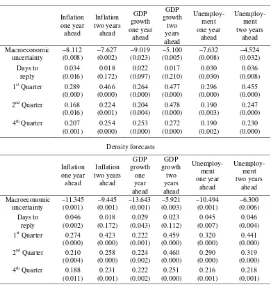
Equation (2) is estimated by maximum likelihood. Table 2 reports the random-effects estimators of the parameters.25 The uncertainty measure, based on the Gini index as described in Section 2, is statistically significant at conventional levels in all the estimated models, rejecting the missing-at-random assumption. As expected, the effect on response from the number of days to reply is statistically significant and positive in the majority of the estimated models. Finally, there are substantial seasonal effects on response, with lower response to Q3 surveys.
The results are qualitatively the same when dynamics in the response dummy are allowed.26 In particular, when the response dummy in the previous survey round is included in the model, following Wooldridge (2005), the effect of aggregate uncertainty on the probability of response is still negative and statistically significant in all estimated models. The only difference in the results is
_________________________
submit forecasts for some forecast horizons than for others, because, for instance, she may not trust equally all the models she used to compute her forecasts.
24 The unobserved individual heterogeneity may or may not be correlated with the independent variables of the model. If it is correlated, the fixed-effects estimator is consistent, because the variables are transformed to get rid of the unobserved heterogeneity before estimation. If the unobserved individual heterogeneity is uncorrelated with the independent variables, the fixed-effects estimator is inefficient (although it is still consistent), while the random-effects estimator is more efficient. The Hausman test (Greene 2008; Hausman 1978) does not reject the null hypothesis of absence of systematic differences between the fixed-effects and the random-effects estimators. Hence, the random-effects estimator seems preferable under this metric.
25 The null hypothesis of equal random effects across individuals is clearly rejected for all the estimated models (p-value=0.000).
that the number of days to reply loses even more statistical significance for inflation forecasts two years ahead.
3.2
The quantitative effect on response from changes in uncertainty
The results in Table 2 show the qualitative effect of changes in macroeconomic uncertainty on response to the SPF but not the quantitative effect. Correlation between uncertainty and response could imply that measures of uncertainty based on SPF data may be biased downwards. This would be the case if the forecasters that feel higher macroeconomic uncertainty reply less, ceteris paribus, than the rest because, for instance, they find the task of forecasting to be relatively more costly in a more uncertain environment. In this context, the estimates of uncertainty computed from the data submitted by the remaining SPF panellists may underestimate the overall degree of uncertainty perceived by the average SPF panellist. Section 4 presents an analysis of this potential bias in the estimates of uncertainty computed with SPF data.
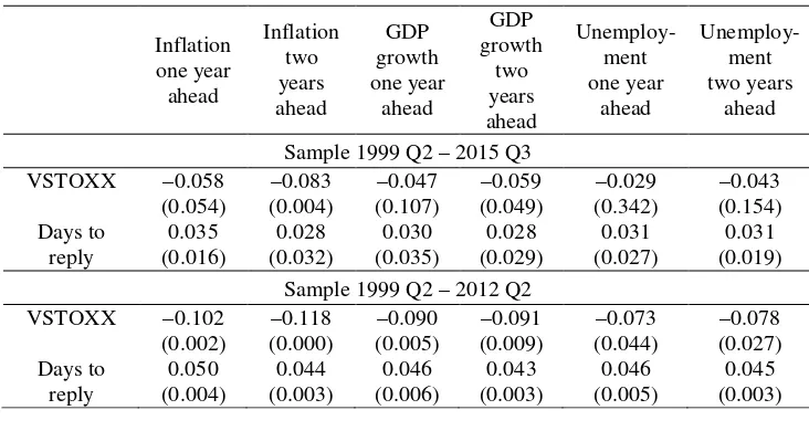
The proper way to quantify the effect of macroeconomic uncertainty on response to the survey requires an estimate of uncertainty that is not computed from the survey itself. Table 3 shows the estimation results of the probit model in (2) using the VSTOXX indices as proxies for macroeconomic uncertainty. For the reasons explained above, I focus on the results for the 1999 Q2–2012 Q2 subsample. Again, the VSTOXX index is always significant, rejecting the missing-at-random assumption. The sign of its coefficient suggests that increases in uncertainty reduced the probability of response at the individual level. This result
is consistent with a production-cost hypothesis (more uncertainty makes
forecasting more costly and reduces the incentives to participate) but not with a strategic-behaviour explanation (forecasters should participate more when it is more likely that their views make a difference for policy).
Table 2: Estimation results of the probit models of response to the SPF using the Gini index as measure of uncertainty
Point forecasts
Table 3: Estimated coefficients of the probit model of response to the SPF using the VSTOXX indices as proxies for macroeconomic uncertainty
Point forecasts
why I trust more the results with the shorter sample but here this conjecture can be substantiated. Figure 8 shows in black the recursive estimates of the VSTOXX coefficient in the model of the probability of submitting point forecasts of unemployment two years ahead using rolling windows of 30 quarters of data. They are roughly constant until end-2012, when they start to increase significantly.27 These recursive estimates may be compared with the recursive estimates using the Gini index to measure uncertainty (in red), which do not change significantly in the last part of the sample. This evidence highlights that something has changed the dynamics of the VSTOXX indices in the last few years and supports the truncation of the sample in 2012 Q2.
Figure 8: Recursive estimates of the coefficient of the uncertainty variable in the model of the probability of submitting point forecasts of unemployment two years ahead
_________________________
Equation (2) makes it clear that the probit model is not linear. Consequently, the estimated coefficients cannot be interpreted as the marginal effects on the dependent variable from changes in the regressors. In general, these marginal effects will vary with the values of the regressors. Figure 9 shows the estimated marginal effects on the probability of response from a one-standard-deviation increase in the VSTOXX index for different values of the index.28 An increase in the VSTOXX by one standard deviation reduces the probability of submitting point and density forecasts by around 3 and 4 percentage points respectively. To put this into perspective, the 4-standard deviation increase in the VSTOXX indices at the start of the financial crisis (from 2007 Q2 to 2009 Q1, see Figure 7) would have reduced the probability of response to the SPF by around 12 percentage points for point forecasts and 16 percentage points for density forecasts. Larger marginal effects for density forecasts than for point forecasts are consistent with the production-cost hypothesis, as density forecasts are typically more difficult to compute than point forecasts.29
These results confirm that ECB’s SPF data is not missing at random. Response to the survey depends negatively on macroeconomic uncertainty, the effect being statistically and quantitatively significant. This finding is evidence in favour of the
production-cost hypothesis: the incentives to reply are lower when uncertainty is higher because the production of forecasts is more costly.
4
Are SPF-based estimates of macroeconomic uncertainty
biased downwards?
Correlation between uncertainty and response could imply that estimates of uncertainty based on SPF data may be biased downwards. This would be the case if the forecasters that feel higher macroeconomic uncertainty reply less, ceteris
_________________________
Figure 9: The marginal effect on the probability of response from changes in uncertainty for different values of the uncertainty measure
Point forecasts
-0.07
Inflation one year ahead
-0.08
Inflation two years ahead
-0.07
GDP growth one year ahead
-0.07
GDP growth two years ahead
-0.07
Unemployment one year ahead
-0.07
Figure 9 (cont.)
Inflation one year ahead
-0.09
Inflation two years ahead
-0.07
GDP growth one year ahead
-0.08
GDP growth two years ahead
-0.08
Unemployment one year ahead
-0.08
paribus, than the rest because, for instance, they find the task of forecasting to be relatively more difficult in a more uncertain environment.
For the estimates of uncertainty based on SPF data to remain unbiased, the panellists that did not reply in more uncertain times had to feel on average the same degree of macroeconomic uncertainty than the panellists that replied. This could be the case if, for instance, higher uncertainty forces some of the participating institutions to disappear: these panellists stopped replying not because it was more difficult to cast their predictions in a more uncertain environment, but because the institution disappeared.
For obvious reasons, the SPF dataset does not allow to check directly whether replying forecasters were less uncertain than non-replying forecasters, as the latter did not submit any data to the ECB. But some indirect evidence supporting the existence of a downward bias in the aggregate measures of macroeconomic uncertainty obtained from the SPF dataset may be found nevertheless.
As preliminary evidence, Figure 10 compares the SPF-based uncertainty measures previously shown on Figure 5 with the 12-month and the 24-month VSTOXX indices. For an easier comparison, all series have been standardised and thereby have zero mean and one standard deviation. The SPF-based uncertainty measures track reasonably well the VSTOXX indices, especially at the two-year horizon, with three notable exceptions. The first and second exceptions are the two biggest spikes in uncertainty according to the VSTOXX indices, which occurred from 2001 Q2 to 2003 Q1 and from 2007 Q2 to 2009 Q1. Over these two periods, uncertainty measures based on SPF data increased by much less than the VSTOXX indices. The third time when financial-based and survey-based measures of uncertainty significantly diverged started in 2012 Q3 and the divergence has persisted until the end of the sample (2015 Q3). During this period, the VSTOXX indices declined significantly but the survey-based measures remained at elevated levels. As indicated above, this phenomenon is probably related to the non-conventional monetary-policy measures taken by central banks, which have had very positive effects on financial markets but less positive effects on the real economy. As a consequence, measures of uncertainty from financial data may be less useful to estimate macroeconomic uncertainty since 2012 Q3.
Figure 10: Comparison between the standardised VSTOXX indices and the standardised SPF-based uncertainty measures from density forecasts one and two years ahead
One year ahead
Two years ahead
12-month VSTOXX Gini (inflation) Gini (GDP growth) Gini (unemployment)
-3
Table 4: Comparison between changes in the standardised 12-month and 24-month VSTOXX indices and the standardised SPF-based uncertainty measures during two
selected episodes
12-month VSTOXX index and SPF uncertainty measures from density forecasts one year ahead
24-month VSTOXX index and SPF uncertainty measures from density forecasts two years ahead
Notes: The cells in the table show the increase in the different measures of uncertainty over the periods on the first column. All uncertainty measures have been standardised. Therefore, the units are standard deviations of each uncertainty measure.
Q1, the VSTOXX indices jumped by 2.65 and 2.77 standard deviations while the SPF-based uncertainty measures increased by much less (by between 0.01 and 1.47 standard deviations). During the second episode, from 2007 Q2 to 2009 Q1, the VSTOXX indices rose by 4.04 and 4.12 standard deviations while the SPF-based uncertainty measures did so by between 0.27 and 1.77 standard deviations only. If we assume that these VSTOXX indices were an accurate indicator of macroeconomic uncertainty in the euro area before 2012 Q3, this finding is consistent with a downward bias in SPF-based uncertainty measures when uncertainty increases.
It could be claimed that this result may have nothing to do with the decision to reply by the forecasters who perceived more uncertainty, but that it is just an indication that professional forecasters became less attentive during the financial crisis and somehow forgot to update the shape of their density forecasts. This is, however, at odds with recent findings by Easaw et al. (2016) who show that
Inflation GDP growth Unemployment
2001Q2 - 2003Q1 2.65 0.45 1.47 0.01
2007Q2 - 2009Q1 4.04 1.21 0.27 0.39
SPF VSTOXX
Inflation GDP growth Unemployment
2001Q2 - 2003Q1 2.77 0.75 0.99 0.17
2007Q2 - 2009Q1 4.12 1.77 1.24 0.60
professional forecasters became more attentive, not less, at times of higher uncertainty.
There is, however, a more rigorous way to obtain evidence on the potential downward bias of SPF uncertainty measures. It is based on the negative relationship between uncertainty and GDP growth, which has been the object of increasing attention since the start of the financial crisis, especially after Bloom’s (2009) seminal paper on the effects of uncertainty shocks.
For instance, Baker and Bloom (2013) found a negative effect of uncertainty shocks on GDP growth rates using natural disasters, terrorist attacks and unexpected political events to identify uncertainty shocks. Popescu and Smets (2010) reported significant negative effects of uncertainty shocks on German business cycles and financial risk premia, but the effects are quantitatively small and temporary. Bloom et al. (2013) used a DSGE model to show that increases in uncertainty may lead to higher returns to inaction by firms: in the presence of labour-adjustment costs, firms reduce net hiring of workers when uncertainty is high, contributing to sharp declines in output and productivity. Arslan el al. (2011) found that uncertainty leads industrial production by around five months due to firms delaying investment projects. Lee et al. (2010) used a VAR framework to find that uncertainty may significantly reduce demand due to precautionary savings.
Interestingly, a few researchers have very recently used the ECB’s SPF data to investigate the relationship between real GDP growth forecasts and measures of uncertainty derived from SPF data. Abel et al. (2015) found a strong negative relationship between uncertainty and aggregate real GDP growth forecasts. They did not use individual data in their analysis. Paloviita and Viren (2014) did use the panel dataset of individual forecasts, finding a negative impact of subjective uncertainty on individual point forecasts of output growth. However, none of these papers controlled for sample selection.
Figure 11: Example on the importance of controlling for sample selection when estimating the effect of subjective uncertainty on individual point forecasts of GDP growth
linear regression line could look like the green line. But if forecasters decide not to reply to the survey when their subjective measure of uncertainty is above a certain threshold, U0, an econometrician that does not control for sample selection could
obtain a linear regression line similar to the yellow line, which overestimates the negative effect of uncertainty on expected GDP growth.
Therefore, evidence on the relationship between individual response and individual perceptions of uncertainty may be obtained by running two regressions. First, regress the individual forecasts of GDP growth on measures of subjective uncertainty ignoring sample selection. Then, do the same controlling for sample selection. If a smaller slope (in absolute value) were obtained when controlling for sample selection, this would be evidence of a lower likelihood of response by the forecasters that perceive more uncertainty.
More formally, I first estimate the following model:
it i it e
it
c
U
g
=
+
β
+
µ
+
η
(4)Subjective uncertainty
G
D
P
gr
ow
th f
or
ec
as
t
where
g
ite is the point forecast of the real GDP growth rate submitted by panellist iduring survey round t, and Uit is the individual Gini index of uncertainty computed
from the panellist’s density forecast.30
i
µ
is an unobservable individualcomponent that is constant over time. c and β are constant parameters, andηit is a
disturbance with zero conditional mean:
[
itU
is,
i]
=
0
E
η
µ
s = 1, 2, …, t,… T (5)Equation (5) is the strict-exogeneity assumption required to estimate models like (4) under fixed or random effects. Abel et al. (2015) and Paloviita and Viren (2014) also assumed that uncertainty is exogenous. Moreover, Bloom et al. (2013) found no significant causal impact of industry growth rates on industry uncertainty, Arslan et al. (2011) support the exogeneity of uncertainty based on Granger causality tests and endogeneity tests, and Haddow et al. (2013) found unidirectional causality from uncertainty measures to confidence indicators.
The top panel in Table 5 shows the fixed-effects estimators of the β parameter in (4) when sample selection is not controlled for. The estimated coefficients are significantly lower than zero for both forecast horizons, suggesting that forecasters perceiving more uncertainty submitted lower GDP-growth forecasts to the ECB.
Estimating (4) with the available SPF data assumes that the response decision is random, i.e. it does not depend on uncertainty. However, the evidence shown in the previous section suggests that response and uncertainty may be correlated. If SPF panellists do not reply when uncertainty is too high, the fixed-effects estimator of (4) may be inconsistent. In order to obtain consistent estimates of β for the population of SPF panellists, and not only for those who reply, two alternatives are available. The first option is to use Wooldridge’s (2007) Inverse-Probability-Weighted estimator. The second is to use Wooldridge’s (1995) two-step procedure based on Inverse Mills Ratios. Unlike the former, the latter requires that selection is based on observables, which is not the case here because the level
_________________________
of uncertainty perceived by each individual is not observable if the forecaster does not respond to the survey. This problem, however, can be solved assuming that:
it t it U
U = +η (6)
This assumption implies that each forecaster perceives a level of uncertainty equal to the aggregate level of uncertainty plus an idiosyncratic measurement error. Under the classical errors-in-variables assumption typically used with measurement errors, ηit is uncorrelated with Ut. Therefore, I will follow
Wooldridge’s (1995) two-step procedure because of its simplicity. 1st step: Estimate the following probit model for each survey round:
Pr(forecaster i submits a GDP point forecast and a density forecast h years ahead)
= Φ
(
β+β1Q1t+β2Q2t+β4Q4t +βUUt +βDDt+ui+εit)
(7)with
it U it it ϑ β η
ε = +
[
it Uis, i]
=0Eϑ µ s = 1, 2, …, t,… T
Equation (7) is similar to the probit model estimated in the previous section, (2), with one exception: following Wooldridge (1995) again, the unobservable individual component in (7),
u
i, is assumed to be a linear combination of the individual Gini indices for t = 1, …, T. In particular, as proposed by Mundlak (1978):∑
==
+
=
t Tt
i it f
i
U
T
u
1
1
ξ
β
(8)where
ξ
iU
it is a normally-distributed disturbance with zero mean and constantvariance. This individual effect is a measure of the individual commitment to participate: ceteris paribus, a more committed forecaster will reply to the survey at times when uncertainty is higher, resulting in a higher ui.
Pr(forecaster i submits a GDP point forecast and a density forecast h years ahead)
The results of these auxiliary regressions are not shown to save space but are available from the author upon request. The only noticeable result is that estimates of βf are typically positive. This is not surprising because the unobservable
individual component captures the commitment to reply by each forecaster. The more commitment, other things equal, the higher the likelihood that the forecaster replies when uncertainty is high and thereby the higher the average subjective uncertainty reported by the forecaster.
2nd step: For each estimated probit model, i.e. for each time period, obtain the
inverse Mills ratios evaluated at
∑
=
forecasters that submitted a GDP growth point forecast and a density forecast h
years ahead. Then construct T auxiliary regressors, each one a 1xT vector:
]
Finally, under the assumption that the conditional expectation of the disturbance in (4) is a linear function of the combined disturbance in (9), as in Wooldridge (1995),
[
itU
is,
i,
v
is]
t(
v
it i)
E
η
µ
=
γ
+
ξ
s=1, 2, …, T. (11)it
by pooled OLS, where
t
it has zero mean conditional on the regressors. Note that,as in (9), the unobservable individual component has been replaced with a linear function of the average subjective uncertainty by forecaster. The results of this estimation are shown in Table 5, bottom panel, although the 65 estimated parameters γt are not shown to save space.31 The estimated slope coefficient of the
relationship between individual uncertainty and GDP growth forecasts, β, is much smaller when sample selection is controlled for. It is actually not significantly different from zero at 5% significance levels. Instead, all the negative effects of uncertainty on growth forecasts go through the individual effect: individuals who perceive higher average uncertainty over time report lower growth forecasts on average.
This result suggests that panelists perceiving higher individual uncertainty are indeed participating less. More evidence on this is presented on Figure 12, that shows in blue the estimated average selection effect,
γ
ˆ
tw
it , i.e. the difference between the expected GDP growth rate by the average replying forecaster and the expected GDP growth rate by the average SPF forecaster. This effect may be interpreted as an estimate of the distance between the yellow line and the green line in Figure 11.The estimated average selection effect is found to be negatively correlated with macroeconomic uncertainty. The upper panels in Figure 12 use the VSTOXX as proxies for uncertainty and the lower panels use the Gini index. During the period with the lowest macroeconomic uncertainty according to the Gini index, at the beginning of the sample, the average selection effect is positive. This means that the yellow line in Figure 11 is above the green line when uncertainty is low. However, the estimated average selection effect quickly became negative when uncertainty increased at the start of the crisis, suggesting that the yellow line lies below the green line when uncertainty is high. The correlation coefficients between the VSTOXX indices and the average selection effect on forecasts of
_________________________
GDP growth one and two years ahead are -0.44 and -0.39 respectively. When the Gini index is used to measure uncertainty these correlations increase to –0.62 to – 0.84.
Overall, the results of the estimated sample-selection models support the hypothesis that the panelists that perceive more uncertainty are less likely to reply to the ECB’s SPF. Therefore, SPF-based aggregate measures of uncertainty which do not control for sample selection are likely to be biased downwards.
Table 5: Estimation of the relationship between individual uncertainty and expected GDP growth with and without controlling for sample selection
Without controlling for sample selection:
g
ite=
c
+
β
U
it+
µ
i+
ε
itNotes: The cells display the fixed-effects estimators of the model parameter β. P-values in
parenthesis based on clustered-robust standard errors. Sample period: 1999 Q1 – 2015 Q3.
Controlling for sample selection:
it
Figure 12: Time series of the estimated average sample-selection effect
With forecasts of GDP growth one year ahead
-3.0
estimated average selection effect (lhs) macroeconomic uncertainty (12-month VSTOXX, rhs)
0.93
Figure 12 (cont.)
With forecasts of GDP growth two years ahead
-3.5
estimated average selection effect (lhs) macroeconomic uncertainty (24-month VSTOXX, rhs)
0.90
5
Conclusions
This paper has explored the link between the degree of macroeconomic uncertainty and the decision to reply to the ECB’s Survey of Professional Forecasters. A discrete-choice model is estimated with panel data to test if changes in uncertainty measures had any effects on the likelihood to reply by SPF forecasters.
The main result of the paper is that data in the ECB’s SPF is not missing at random as higher (lower) uncertainty reduces (increases) response to the survey. This effect is statistically and economically significant. For instance, the increase in macroeconomic uncertainty at the start of the financial crisis (2008–2010) reduced the probability of response by SPF participants by around 12 percentage points for point forecasts and by around 16 percentage points for density forecasts. This finding has implications for the information content of ECB’s SPF data. Given that fewer replies are likely to be received when uncertainty surges, the information content of the survey may be eroded during periods of heightened uncertainty, precisely when the information from the survey may be needed the most. Moreover, Kenny et al. (2015) showed that prudent forecasters, i.e. those who perceive more uncertainty, exhibit a better forecasting track record. If these forecasters are less likely to reply when uncertainty increases, the worst-performing forecasters may become over-represented in the ECB’s SPF sample and, then, the ECB’s SPF aggregate forecasts would become less informative and reliable.
Furthermore, if forecasters perceiving more uncertainty are less likely to reply, the estimates of uncertainty based on the data submitted by the remaining panellists may underestimate the overall degree of uncertainty perceived by SPF panellists. A comparison between the estimated parameters of a relationship between subjective uncertainty and individual GDP-growth forecasts, with and without controlling for sample selection, yields results that are consistent with the hypothesis that panellists facing more uncertainty are less likely to reply to the survey. Consequently, measures of uncertainty from the ECB’s SPF typically used in the literature could be biased downwards.
could be fine-tuned to minimise the exit of panellists. And if attrition turns out to be correlated with economic developments, these could induce time-variation in the information content of the survey.
References
Abel, J., Rich, R., Song, J., and Tracy, J. (2015). The measurement and behaviour of uncertainty: Evidence for the ECB survey of professional forecasters. Forthcoming in the Journal of Applied Econometrics.
http://onlinelibrary.wiley.com/doi/10.1002/jae.2430/abstract
Arslan, Y., Atabek, A., Hülagü, T., and Șahinöz, S. (2011). Expectation errors, uncertainty and economic activity. Central Bank of the Republic of Turkey Working Paper, 11/17.
http://www.tcmb.gov.tr/wps/wcm/connect/ca940d40-a081-49ce-9d07-60b1e7f210d6/WP1117.pdf?MOD=AJPERES&CACHEID=ROOTWORKSPACEca 940d40-a081-49ce-9d07-60b1e7f210d6
Baker, S.R., and Bloom, N. (2013). Does uncertainty reduce growth? Using disasters as natural experiments. NBER Working Paper, 19475.
http://www.nber.org/papers/w19475
Bekaert, G., Hoerova, M., and Lo Duca, M. (2013). Risk, uncertainty and monetary policy.
Journal of Monetary Economics 60(7): 771–788.
http://www.sciencedirect.com/science/article/pii/S0304393213000871
Bloom, N. (2009). The impact of uncertainty shocks. Econometrica 77(3): 623–685.
http://onlinelibrary.wiley.com/doi/10.3982/ECTA6248/abstract
Bloom, N., Floetotto, M., Jaimovich, N., Saporta-Eksten, I., and Terry, S. J. (2013). Really uncertain business cycles. CEP Discussion Paper, 1195.
http://cep.lse.ac.uk/pubs/download/dp1195.pdf
Bowles, C., Friz, R., Genre, V., Kenny, G., Meyler, A., and Rautanen, T. (2010). An evaluation of the growth and unemployment forecasts in the ECB survey of professional forecasters. Journal of Business Cycle Measurement and Analysis 4(2): 1–28.
http://www.oecd-ilibrary.org/economics/an-evaluation-of-the-growth-and- unemployment-forecasts-in-the-ecb-survey-of-professional-forecasters_jbcma-2010-5km33sg210kk
Conflitti, C. (2011). Measuring uncertainty and disagreement in the European survey of professional forecasters. Journal of Business Cycle Measurement and Analysis 7(2): 69–103.
http://www.oecd-ilibrary.org/economics/measuring-uncertainty-and-disagreement-in-the-european-survey-of-professional-forecasters_jbcma-2011-5kg0p9zzp26k
Den Van Berg, G.J., Lindeboom, M., and Ridder, G. (1994). Attrition in longitudinal panel-data and the empirical analysis of dynamic labour-market behaviour. Journal of Applied Econometrics 9(4): 421–435.
Easaw, J., Golinelli, R., and Heravi, S. (2016). Inflation forecasts, inattentiveness and uncertainty. Presented at the 36th International Symposium on Forecasting, Santander, June.
ECB (2014a). Fifteen years of the ECB survey of professional forecasters. ECB Monthly Bulletin, January: 55–67.
https://www.ecb.europa.eu/pub/pdf/other/art1_mb201401en_pp55-67en.pdf
ECB (2014b). Results of the second special questionnaire for participants in the ECB survey of professional forecasters. Retrieved on 24 May 2015 from
http://www.ecb.europa.eu/stats/prices/indic/forecast/shared/files/resultssecondspecialq uestionnaireecbsurveyspf201401en.pdf??92f09eaa6906c6e15bf77fb4dcdd055f
ECB (2014c). Results of the ECB survey of professional forecasters for the first quarter of 2014. ECB Monthly Bulletin, February: 60–65.
https://www.ecb.europa.eu/pub/pdf/other/mb201402_focus08.en.pdf
Engelberg, J., Manski, C.F., and Williams, J. (2011). Assessing the temporal variation of macroeconomic forecasts by a panel of changing composition. Journal of Applied Econometrics 26(7): 1059–1078.
http://onlinelibrary.wiley.com/doi/10.1002/jae.1206/abstract
Gini, C. (1955). Variabilità e mutabilità. In E. Pizzeti and T. Salvemini (Eds.), Memorie di metodologica statistica. Rome: Libreria Eredi VirgilioVeschi.
Glas, A., and Hartmann, M. (2016). Inflation uncertainty, disagreement and monetary policy: Evidence from the ECB Survey of Professional Forecasters. Forthcoming in the Journal of Empirical Finance.
http://www.sciencedirect.com/science/article/pii/S092753981630041X
Gómez, V., and Maravall, A. (2001). Seasonal adjustment and signal extraction in economic time series. In D. Peña, G.C. Tiao and R.S. Tsay (Eds.), A Course in Time Series Analysis. John Wiley & Sons.
http://onlinelibrary.wiley.com/book/10.1002/9781118032978
Greene, W. H. (2008). Econometric Analysis. Pearson/Prentice Hall.
Haddow, A., Hare, C., Hooley, J., and Shakir, T. (2013). Macroeconomic uncertainty: what is it, how can we measure it and why does it matter? Bank of England Quarterly Bulletin, 2013 Q2: 100–109.
http://www.bankofengland.co.uk/publications/Documents/quarterlybulletin/2013/qb1 30201.pdf
Hausman, J.A. (1978). Specification tests in econometrics. Econometrica 46(6): 1251– 1271.