Endomiru kako ni okeru bari yosoku shisutemu no kaihatsu
Bebas
122
0
0
Teks penuh
(2) A Thesis for the Degree of Ph.D. in Engineering. Development of Burr Prediction System for End Milling. July 2015 Graduate School of Science and Technology Keio University. KRUY, Sothea.
(3) Development of Burr Prediction System for End Milling. July 2015. A thesis submitted in partial fulfilment of the requirements for the degree of Doctor of Philosophy in Engineering. Keio University Graduate School of Science and Technology School of Integrated Design Engineering. KRUY, Sothea.
(4) Table of Contents List of Figures ...............................................................................................................................iv List of Tables ..................................................................................................................................viii ACKNOWLEDGMENT........................................................................................................ix ABSTRACT ..................................................................................................................................x 1. Motivation and Introduction ...........................................................................................1 1.1 Overview of issues regarding burrs ........................................................................................1 1.2 Significance of research ...........................................................................................................2 1.3 Research objectives ..................................................................................................................3 1.4 Organization of dissertation .....................................................................................................3. 2. Literature Review ..................................................................................................................5 2.1 Burr descriptions and classification ........................................................................................5 2.1.1 Burr definitions ...............................................................................................................5 2.1.2 Burrs from milling operations .......................................................................................6 2.2 Mechanics of burr formation ...................................................................................................10 2.2.1 Poisson burr model .........................................................................................................10 2.2.2 Rollover burr model .......................................................................................................12 2.3 Parameters that influence burr formation ...............................................................................18 2.4 Burr measurement ....................................................................................................................19 2.5 Chapter summary ......................................................................................................................20. 3. Burr Prediction Method ....................................................................................................21 3.1 Classification of burrs in end milling ......................................................................................21 3.1.1 Entrance burr ...................................................................................................................22 3.1.2 Entrance side burr ...........................................................................................................22 3.1.3 Top burr ............................................................................................................................23 3.1.4 Exit burr ............................................................................................................................23 3.1.5 Exit side burr ...................................................................................................................24 3.2 Application of burr models in end milling .............................................................................24 3.2.1 Entrance burr model in up milling .................................................................................24 3.2.2 Entrance burr model in down milling ...........................................................................26. i.
(5) 3.2.3 Entrance side burr model in up milling and down milling...........................................27 3.2.4 Top burr model in up milling and down milling ..........................................................27 3.2.5 Exit burr model in up milling and down milling ..........................................................28 3.2.6 Exit side burr model in up milling and down milling ..................................................30 3.3 Chapter summary ......................................................................................................................31. 4. Development of Burr Prediction System ..................................................................32 4.1 System architecture ...................................................................................................................32 4.2 Geometric simulation ...............................................................................................................33 4.2.1 Z-map model ....................................................................................................................33 4.2.2 NC program analysis model ...........................................................................................36 4.3 Physical simulation ...................................................................................................................37 4.3.1 Cutting length calculation ...............................................................................................37 (1) Entrance pattern .........................................................................................................37 (2) Ready pattern .............................................................................................................38 (3) Exit pattern .................................................................................................................39 4.3.2 Axial and radial depth of cut calculation .......................................................................41 4.3.3 Cutting area calculation ...................................................................................................44 4.3.4 Cutting force calculation ..................................................................................................45 (1) First method of cutting forces calculation ...............................................................45 (2) Second method of cutting forces calculation ..........................................................47 4.4 Burr prediction ..........................................................................................................................50 4.4.1 Identification of burr formed by NC simulation...........................................................50 4.4.2 Identification of top burrs and applied formula ...........................................................50 4.4.3 Identification of exit burrs and applied formula ..........................................................53 4.4.4 Identification of exit side burrs and applied formula ..................................................54 4.4.5 Identification of entrance burrs and applied formula ..................................................56 4.4.6 Identification of entrance side burrs and applied formula ..........................................57 4.4.7 Burr direction ..................................................................................................................58 4.5 Execution of burr prediction system .......................................................................................59 4.5.1 Method for operating burr prediction system ...............................................................59 4.6 Tool path planning for burr minimization...............................................................................62 4.6.1 Basic tool path planning ..................................................................................................62. ii.
(6) 4.6.2 Other tool path planning cases .......................................................................................66 4.7 Burr prediction based on flank wear during end milling ......................................................68 4.8 Chapter summary .....................................................................................................................70. 5. System Verification ...............................................................................................................71 5.1 Simulation of burr formation in end milling ..........................................................................71 5.2 Experimental verification..........................................................................................................74 5.2.1 Evaluation method for burr generation using fresh cutting tool .................................74 5.2.2 Evaluation method for burr generation using cutting tool with flank wear................91 5.3 Discussion ..................................................................................................................................96 5.3.1 Burr results using first method of cutting force calculation .........................................96 5.3.2 Burr results using second method of cutting force calculation ...................................97 5.3.3 Comparison between first method and second method of cutting force calculation.97 5.3.4 Burrs results using cutting tool with flank wear ...........................................................98 5.3.5 Effects of radial depth of cut, axial depth of cut, and feed rate on exit side burr and top burr .............................................................................................................................98 5.4 Chapter summary ......................................................................................................................100. 6. Conclusion .................................................................................................................................101 6.1 Conclusion......................................................................................................................................101 6.2 Future research ...............................................................................................................................103. BIBLIOGRAPHY ......................................................................................................................104 LIST OF ACHIEVEMENTS ..............................................................................................107. iii.
(7) List of Figures Fig. 1.1 Share of manufacturing effort caused by burrs7) .............................................................. 3 Fig. 2.1 Definitions and geometry of a burr6), 7) .............................................................................. 6 Fig. 2.2 Five types of burrs observed in face milling2) .................................................................. 7 Fig. 2.3 Identification of burr locations in end milling1) ................................................................ 8 Fig. 2.4 Relationship between chip flow angle and region chip deformation8)........................... 8 Fig. 2.5 Exit order and burr formation process8)............................................................................. 9 Fig. 2.6 Poisson burr formed when cutting tool pushed into workpiece9) ................................. 11 Fig. 2.7 Rollover burr formation process4) .................................................................................... 13 Fig. 2.8 SEM microphotograph at initiation state of burr formation2) ...................................... 15 Fig. 2.9 Rollover burr that occurs when cutting tool exits workpiece9) ..................................... 15 Fig. 2.10 Schematic illustration of oblique cutting3) .................................................................... 17 Fig. 2.11 Interdependencies of burr formation parameters7) ....................................................... 18 Fig. 2.12 Methods of burr detection and measurement7) ............................................................. 19 Fig. 3.1 Locations of burrs shown in red for end milling process. ............................................. 21 Fig. 3.2 Entrance burr location . ..................................................................................................... 22 Fig. 3.3 Entrance side burr location . ............................................................................................. 22 Fig. 3.4 Top burr location . ............................................................................................................. 23 Fig. 3.5 Exit burr location . ............................................................................................................. 23 Fig. 3.6 Exit side burr location . ..................................................................................................... 24 Fig. 3.7 Bottom view of end milling tool . .................................................................................... 25 Fig. 3.8 Detail of bottom view of end milling tool in up milling ............................................... 25 Fig. 3.9 Detail of bottom view of end milling tool in down milling . ........................................ 26 Fig. 3.10 Side view of shoulder end milling9) .............................................................................. 27 Fig. 3.11 Top burr formed in down milling . ................................................................................ 28 Fig. 3.12 Top burr formed in up milling ......................................................................................28 Fig. 3.13 Rollover burr formed when cutting depth is large . ..................................................... 29 Fig. 3.14 Rollover burr formed at side edge by multiple cuts . ................................................... 30 Fig. 3.15 Locations of burrs in shoulder end milling9) ................................................................ 31 Fig. 4.1 Numerical calculation process . ....................................................................................... 33 Fig. 4.2 Boolean subtraction with Z-map model . ........................................................................ 34. iv.
(8) Fig. 4.3 Z-map model used to represent workpiece9) .................................................................. 35 Fig. 4.4 Cutting length in each segment at entrance pattern of cutting tool . ............................ 38 Fig. 4.5 Cutting length in each segment at ready pattern of cutting tool . ................................. 39 Fig. 4. 6 Cutting length in each segment at exit pattern of cutting tool ..................................... 40 Fig. 4.7 Method for calculating radial depth of cut . .................................................................... 41 Fig. 4.8 Method for distinguishing areas A and B . ..................................................................... 42 Fig. 4.9 Method for calculating radial depth of cut . .................................................................... 43 Fig. 4.10 Flowchart for calculating radial depth of cut . .............................................................. 44 Fig. 4.11 Cutting force definition for tool rake face9) . ................................................................ 46 Fig. 4.12 Cutting force model in up milling26) ............................................................................. 47 Fig. 4.13 Grid point coordinate and interference point Ip …………………………………..51 Fig. 4.14 Judgment of burr type using Z-map height of grid point coordinate and Z-map height of interference point Ip . .................................................................................................................. 51 Fig. 4.15 Burr direction condition . ................................................................................................ 58 Fig. 4.16 Input data screen for system execution . ....................................................................... 59 Fig. 4.17 Console window screen for system execution . ........................................................... 60 Fig. 4.18 Console window screen for system execution to predict burr location and size …..61 Fig. 4.19 Console window screen for system execution with complex shape . ........................ 61 Fig. 4.20 Tool path planning in down milling adapted window frame method26) . .................. 62 Fig. 4.21 Tool path planning modified to avoid exit burr . ......................................................... 63 Fig. 4.22 Exit burr formed in case of cutting tool engaged from inside . .................................. 64 Fig. 4.23 Three types of tool paths in down milling26) ................................................................ 65 Fig. 4.24 Tool path method for tool path C26) . ............................................................................. 65 Fig. 4.25 Tool path method when workpiece width is smaller than tool diameter . ................. 66 Fig. 4.26 Tool path method when workpiece has round shape . ................................................ 67 Fig. 4.27 Cutting force model due to flank wear ......................................................................... 69 Fig. 5.1 Cutting tool 2SSD1000S10 and its detailed geometry12) .............................................. 74 Fig. 5.2 Machine center MSA30 Seiki Makino .......................................................................... 75 Fig. 5.3 Workpieces for testing ..................................................................................................... 76 Fig. 5.4 Digital microscope (KEYENCE: VHX-600) was used to measure average exit burr size .................................................................................................................................................... 77. v.
(9) Fig. 5.5 Image of entrance burr in up milling for gray cast iron 250 enlarged by digital microscope . ..................................................................................................................................... 78 Fig. 5.6 Image of entrance side burr in up milling for gray cast iron 250 enlarged by digital microscope . ..................................................................................................................................... 78 Fig. 5.7 Image of entrance burr in up milling for stainless steel 6 enlarged by digital microscope . ........................................................................................................................................................... 78 Fig. 5.8 Image of entrance burr in up milling for AlMg0.5Si enlarged by digital microscope. ........................................................................................................................................................... 79 Fig. 5.9 Image of entrance burr in down milling for steel C: 0.45 % enlarged by digital microscope . ..................................................................................................................................... 79 Fig. 5.10 Image of entrance burr in up milling for steel C: 0.45 % enlarged by digital microscope . ..................................................................................................................................... 79 Fig. 5.11 Comparison of top burrs in up milling of steel C : 0.45% . ........................................ 80 Fig. 5.12 Comparison of top burrs in down milling of steel C: 0.45 % . ................................... 80 Fig. 5.13 Comparison of exit burrs in cutting direction of steel C: 0.45 % . ............................. 81 Fig. 5.14 Comparison of exit burrs in feed direction of steel C: 0.45 % ................................... 81 Fig. 5.15 Comparison of top burrs in down milling of gray cast iron 250 . .............................. 82 Fig. 5.16 Comparison of top burrs in down milling of stainless steel 6 .................................... 82 Fig. 5.17 Comparison of entrance burrs in down milling of steel C: 0.45 % . .......................... 83 Fig. 5.18 Comparison of top burrs in up milling of steel C: 0.45 % . ........................................ 83 Fig. 5.19 Comparison of top burrs in down milling of steel C: 0.45 % . ................................... 84 Fig. 5.20 Comparison of exit burrs in up milling of steel C: 0.45 % . ....................................... 84 Fig. 5.21 Comparison of exit burrs in down milling of steel C: 0.45 % . .................................. 85 Fig. 5.22 Comparison of exit burrs in up milling of AlMg0.5Si . .............................................. 85 Fig. 5.23 Comparison of exit burrs in down milling of AlMg0.5Si . ......................................... 86 Fig. 5.24 Burr simulation for complex shape . ............................................................................. 86 Fig. 5.25 Detailed dimensions of complex shape ........................................................................ 87 Fig. 5.26 Tool path A in down milling (burr height = 200 μm) ................................................. 88 Fig. 5.27 Tool path B in down milling (burr height = 50 μm) . .................................................. 88 Fig. 5.28 Tool path C in down milling (burr height = 500 μm) . ................................................ 89 Fig. 5.29 Tool path A in up milling (burr height = 1000 μm) . .................................................. 89 Fig. 5.30 Tool path B in up milling (burr height = 800 μm) . ................................................... 90. vi.
(10) Fig. 5.31 Tool path C in up milling (burr height = 1500 μm) . ................................................... 90 Fig. 5.32 Tool flank wear left to right 0.1 mm, 0.2 mm, and 0.3 mm ....................................... 91 Fig. 5.33 Measurement of exit burr for steel C: 0.45 % workpiece material in test number 1 using tool with 0.1 mm of flank wear ........................................................................................... 92 Fig. 5.34 Comparison of exit burrs of steel after tool wear of 0.1 mm . .................................... 93 Fig. 5.35 Comparison of exit burrs of steel after tool wear of 0.2 mm . .................................... 93 Fig. 5.36 Comparison of exit burrs of steel after tool wear of 0.3 mm . .................................... 93 Fig. 5.37 Comparison of exit burrs of AlMg0.5Si after tool wear of 0.1 mm .......................... 93 Fig. 5.38 Comparison of exit burrs of AlMg0.5Si after tool wear of 0.2 mm .......................... 93 Fig. 5.39 Comparison of exit burrs of AlMg0.5Si after tool wear of 0.3 mm .......................... 93 Fig. 5.40 Effect of radial depth of cut on exit side burr for workpiece material steel C: 0.45 % . ........................................................................................................................................................... 93 Fig. 5.41 Effect of axial depth of cut on burr thickness of top burr for workpiece material steel C: 0.45 % . ....................................................................................................................................... 93 Fig. 5.42 Effect of feed rate on burr thickness of top burr for workpiece material steel C: 0.45 % . ........................................................................................................................................................... 93. vii.
(11) List of Tables Table 3.1 Classification for use of burr models ............................................................................ 31 Table 4.1 G-code functions15) ......................................................................................................... 36 Table 5.1 Different cutting conditions used in tests on steel C:0.45% ...................................... 71 Table 5.2 Different cutting conditions used in tests on AlMg0.5Si .......................................... 72 Table 5.3 Different cutting conditions used in tests on gray cast iron 250 ................................ 72 Table 5.4 Different cutting conditions used in tests on stainless steel 6 ................................... 73 Table 5.5 Workpiece material property25) ..................................................................................... 73 Table 5.6 Cutting tool parameters ................................................................................................. 74 Table 5.7 Evaluation of three tool types ....................................................................................... 87 Table 5.8 Different cutting conditions used in tests on tool with flank wear ............................ 92 Table 5.9 Workpiece material properties25) .................................................................................. 92. viii.
(12) ACKNOWLEDGMENT I would like to express my deepest gratitude and most sincere appreciation to Professor Hideki Aoyama, my research advisor and the chairperson of my dissertation committee, for his continuous support and exceptional guidance throughout this challenging and rewarding research work. His comments and advice during the research have contributed immensely toward the success of this study.. I am also indebted to my thesis co-supervisors: Professor Tojiro Aoyama, Professor Yan Jiwang, and Associate Professor Yasuhiro Kakinuma for reviewing the manuscript and providing me with helpful suggestions and comments. My gratitude also goes to Associate Professor Tetsuo Oya for his support in my study.. I also thank the Japan International Cooperation Agency (JICA) for the scholarship and financial support during my three years of study in Japan. My sincere gratitude also goes to the staff of the ASEAN University Network/ Southeast Asia Engineering Development Network (AUN/ SEED-Net) for their indirect support throughout these years.. I would like to thank Keio University for providing a sufficient environment and facilities to support my study. My warmest regard goes to every member of the Hideki Aoyama laboratory, both the graduates and undergraduates.. Last, but not least, my gratitude goes to my parents (Kruy, Chheangtech and Tan, Muyim), and my financer (Oum, Boramey), for their loving encouragement and best wishes throughout the period of this study.. July 10, 2015. Kruy, Sothea. ix.
(13) ABSTRACT In modern industry, the precision of machined workpiece plays important roles in the industrial applications. Edge imperfections are often introduced on workpiece as a result of plastic deformation during machining. These imperfections are known as burrs. A burr has been basically defined as a thin ridge or area of roughness produced when cutting or shaping metal. A burr leads to an undesirable workpiece edge that must be removed to enhance the level of precision of the part. This not only lowers the production quality, but also causes various problems such as attachment errors or mechanical problems. Thus, deburring processes are needed. However, even with the current sophisticated automation of production processes, deburring is often done by hand, and is a large obstacle to raising the efficiency of manufacturing processes. In addition, the cost of deburring a precision workpiece can be a significant addition to the cost of the finished parts. Thus, the control of burr formation is a research topic of great significance for industrial applications.. Predicting the positions and dimensions of burrs can be used as a countermeasure. This prediction can not only automate the deburring process but can also be applied to perform tool paths testing to reduce burr. Traditional studies on burr prediction have been based on experimental data. These methods are effective in processing methods with a limited number of parameters. However, they are not practical for complex machining with many parameters such as end milling, which would require large amount of experimental data for all its parameters.. In this paper, a system is proposed that uses a machining simulation to predict the positions and dimensions of burr in the end milling process as a preventive method. This system is based on burr formation models, the cutting conditions, and analytical cutting force mode. This system does not require a large quantity of experimental data like the systems used in traditional studies. Two kinds of burr models were used: rollover burr and Poisson burr. Orthogonal and oblique cuts were also applied in the system based on different positions. A Windows based program was developed to illustrate the machining process using a PC-based numerical control (NC) simulator that consisted of a geometric simulator and physical. x.
(14) simulator. The geometric simulator utilized feature identification and cutting condition identification. The physical simulator contained a cutting force model that was used to calculate the force in the feed direction that led to burr form. The proposed system was compared with experimental data for different workpiece materials for validation. It was verified that top and exit burrs could be predicted in up milling and down milling. The predicted and experimental results were found to agree under most of cutting conditions. In addition, a tool path planning scheme was included in the system to avoid tool exits. This method provides a feasible way of suppressing exit burr formation in an automatic manner, and thus reduces the need for deburring. Moreover, the results of a study of the burr size variation based on the tool flank wear in relationship to the cutting edge radius wear are also discussed. This study can be summarized as follows.. 1. A burr prediction method for end milling was proposed based on an examination of the motion and shape of the cutting tool in two burr models for two-dimensional orthogonal cutting and three-dimensional oblique cutting. 2. A prediction method was developed for the thickness and height of a burr based on the burr formation mechanisms and calculation of the cutting force module using a cutting constant in end milling. 3. The usefulness of the burr prediction method and system was verified by performing cutting experiments in several kinds of material with a machining center (milling machine). It was verified that both the predicted and experimental results were found to agree under most of cutting conditions. 4. A method for tool path planning under a window framing scheme was proposed for burr minimization. The entrance burr for tool path in down milling seemed to be reduced burr size, but machine time was increased. The window framing method with roll-ending technique in down milling is a good method to avoid tool exit, thus minimizing burr. 5. A new model was proposed to understand the burr formation and tool wear behavior of a solid carbide tool during dry end milling. The tool flank wear was shown to have significant influence on the cutting force, and increase in cutting resulted in a substantial increase in the burr size.. xi.
(15) CHAPTER 1. 1. Motivation and Introduction. 1.1 Overview of issues regarding burrs In recent years, advances in computer technology have been introduced in manufacturing processes in order to improve manufacturing techniques in response to the demands placed by designers on workpiece performance and functionality. The computers behind these techniques, such as computer aided design (CAD), computer aided manufacturing (CAM), manufacturing planning and control systems (MP & CS), automated materials handling (AMH), flexible manufacturing systems (FMS) and robotics, have been used for easier communication between humans and machines. Recently, these techniques have focused on the development of computer integrated manufacturing (CIM); however, some specific areas such as cleaning, deburring, and surface finishing have not drawn much attention.. In the manufacturing environment, a burr has been defined as an excess of material beyond the edge of a workpiece as a result of the plastic deformation that occurs in cutting and shearing operations. Precision, high productivity manufacturing often requires a deburring or finishing operation. Burrs, together with chips, have been among the most troublesome obstacles to high productivity and the automation of machining processes. The current deburring methods involve manual operations or additional machining with abrasive or finishing tools. Although these are workable solutions, there have several limitations. They are tedious and time consuming. Deburring is usually the last process performed during part production. Thus, it can damage a part with high value or produces an undesirable part dimension. In addition, precautions have to be taken to ensure the safety of workers during the deburring process.. 1.
(16) In the early 1970s, researchers gave much attention to the study of burr formation and deburring techniques. Many methods have been suggested to minimize burr formation or remove burrs. Gillespie and Blotter1) were among the first researchers to study burr formation. They pointed out that deburring and edge finishing on precision workpieces may constitute as much as 30% of the part cost. They believed that burr technology was complex and it required academic excellence, as well as industrial experience. They classified the basic burr formation mechanisms into four basic types, the Poisson, rollover, tear, and cut-off burr formation mechanisms, using an approximation based on the classical plastic deformation mechanism. Other researchers have studied the costs associated with burrs and the basic mechanism for burr formation in machining. The German automotive and machine tool industries showed the costs of burr minimization, deburring, and part cleaning. In their study, the increased costs from burrs were caused by manpower and cycle time increases of about 15%, a 2% share in the rejection rate, and a 4% share in the machine breakdown times7), as shown in Fig. 1.1. Chern and Dornfeld2) and Ko and Dornfeld3) gave more details for a rollover model in orthogonal and oblique cutting. Hashimura et al.4) and Park and Dornfeld5) conducted research analyses of the burr formation mechanism in orthogonal cutting including the influence of material properties based on a simulated analysis using the finite element method (FEM). Hashimura et al.4) also provided schematic views of the burr formation mechanism in different types of workpiece materials, including both ductile and brittle materials. Ota et al.17) proposed the basic burr prediction system; however, their study conducted only for basic shape and the cutting force model was based on cutting constant, which was determined through an experimental test. They did not proposed any specific method for tool path planning for burr minimization or consider the flank wear effect on burr formation.. 1.2 Significance of research Although several researchers have expressed a desire to understand the formation of burrs in more detail, it is not possible to accurately predict the burr size and location using the basic burr formation models. However, embedding a combination of databases on burr properties and burr formation models in a system would make it possible to predict the burrs sizes and locations on precision components. This system could inform the designer or production planner of the effect of certain design changes on the potential for burr formation,. 2.
(17) which should make it possible to reduce the occurrence and severity of burrs on precision components.. Fig. 1.1 Share of manufacturing effort caused by burrs7).. 1.3 Research objectives To date, various methods1,2,3,4,5) have been proposed for the development of burr prediction systems; however, there is no unique system that can be used as a preventive method and that can be applied in practical use. The objective of this thesis is to develop a system for predicting the positions and dimensions of the burrs formed, along with tool path planning for burr minimization and a model to predict the burrs cause by flank wear in the end milling process. This system is a represented in a CAD framework to illustrate the machining process upon a PC-based NC simulator that includes a database of workpiece material properties, tool geometry data, a cutting force model, cutting conditions, and a burr formation model. That information was applied to predict the burr positions and dimensions. Using this approach makes it possible to optimize the factors that affect burr formation, and thus burrs can be minimized.. 1.4 Organization of dissertation Chapter 1 gives an overview of the issues regarding burrs and the significance of this research, along with the objective of this study. A short review of the previous research on burr formation also given.. 3.
(18) Chapter 2 provides background information on burr formation, including burr definitions, and describes the burrs from milling operations, mechanics of burr formation, and analytical models. In addition, burr classification is introduced, along with the types of burrs, parameters that influence burr formation, and burr measurement. The details of two kinds of burr models, the Poisson and rollover burr models, are presented.. Chapters 3 and 4 describe the burr prediction method and development of a burr prediction system. The system architecture of the burr development system in end milling is also illustrated. The development of a geometric simulator is proposed, including a Z-map model, an NC program analysis model, and the identification of up milling and down milling. A physical simulator method is proposed that utilizes three cutting states. A mechanistic forces model, which is an important factor influencing burrs, is illustrated in detail. The identification of the burrs formed in an NC simulation is also explained, and the burr models are applied in end milling. A study was conducted on tool path planning for burr minimization. The influence of the flank wear on burr formation was identified using a cutting edge radius wear analytical model.. In order to verify the proposed burr prediction system for end milling, machining experiments had to be conducted under various cutting conditions. Chapter 5 describes ten experiments that were conducted with a new end milling tool, along with another ten experiments using an end milling tool with flank wear. The experiments were conducted using different kinds of workpiece materials, including steel with 0.45% carbon, aluminum alloy AlMg0.5Si, gray cast iron 250, and stainless steel 6 in 20×20×30-mm sections. The discussion describes the influence of these conditions on the burr sizes. Experimental tests were also conducted to evaluate the burr prediction relation to the flank wear in the end milling. A summary of the thesis is given in chapter 6.. 4.
(19) CHAPTER 2. 2. Literature Review. 2.1 Burr descriptions and classification 2.1.1 Burr definitions In the Oxford English Dictionary, a burr is described as a rough ridge or edge left on metal or another substance after cutting, punching, etc.; e.g., the roughness produced on a copper plate by the graver, the rough neck left on a bullet in casting, or the ridge left on paper, etc. by a puncture. In most cases, a burr is defined as a thin ridge or area of roughness produced in cutting or shaping metal. According to ISO 137156), the edge of a workpiece is defined as having a burr when it has an overhang greater than zero, as shown in Fig. 2.1 (c). Chern and Dornfeld2) defines a burr as the plastically deformed material left and attached to a workpiece after machining. Based on Ko’s finding3), a burr was defined as an “undesirable projection of material formed as the result of plastic flow from a cutting or shearing operation.” Thus, a burr has been defined as an excess of material beyond the edge of a workpiece as a result of the plastic deformation that occurs in cutting and shearing operations. A burr’s geometry was defined by Aurich et al.7), as shown in Fig. 2.1 (a) and (b). He described basic burr parameters using a random cross-section as follows: . The burr root bf : the thickness of the burr root. . The burr height ho: the distance between the ideal edge of the workpiece and the highest point in the cross section. . The burr root radius rf : the radius of a circle positioned at the burr root. . The burr thickness bg : the thickness parallel to the burr root area at a distance of rf. 5.
(20) (a) Burr geometry7). (b) Burr profile in cross direction7). (c) Definitions of burrs according to ISO 137156). Fig. 2.1 Definitions and geometry of a burr6),7).. 2.1.2 Burr from milling operations The type of burr found in face milling operations was observed by Chern and Dornfeld2) to be dependent on the in-plane exit angle. He reported five types of burrs, as illustrated in Fig. 2.2: (a) the knife-type burr, (b) curl-type burr, (c) wave-type burr, (d) edge breakout, and (e) secondary burr.. An end mill can produce eight different burrs in a single slotting operation. These burrs all occur on different edges. For example, in a bottom cutting profiling operation, six edges are produced, and a different group of burrs occurs on each edge, as shown in Fig. 2.3. Gillespie and Blotter1) classified slot milling according to the burr locations, burr shapes and burr formation mechanisms. An exit burr forms when the minor edge of the tool moves away from the workpiece edge. A side burr is defined as occurring on the major edge of the tool cut side surface of the workpiece, and a top burr is defined as a burr attached to the top surface of the 6.
(21) workpiece edge. In Figure. 2.3, the burrs along edges 3, 7, and 9 are the results of chips rolling over, rather than having been sheared from the workpiece1). The burrs on edges 1, 2, and 10 are the results of lateral deformation due to Poisson’s ratio. The burrs along edges 4 and 6 result from material flowing in a direction 180o away from the direction of tool travel. The burrs along edges 8 and 5 vary noticeably along each edge. These are combinations of entrance and rollover burrs.. Fig. 2.2 Five types of burrs observed in face milling2).. Gillespie and Blotter1) also conducted a basic study on the exit side burr along edge 3 shown in Fig. 2.3. They stated that this burr formed based on multiple cuts of the cutter teeth rubbing numerous tightly stacked flaps of material, causing it to roll over repeatedly until the burr fully formed. They showed that the height of this burr is directly proportional to the radial depth of cut as and approximately 0.6 times the cutter diameter. At this radial depth of cut, the material ahead of the cutter tears. Thus, the rollover burr height can be up to 0.6 times the cutter diameter.. 7.
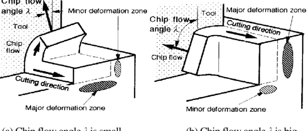
(22) Fig. 2.3 Identification of burr locations in end milling1).. (a) Chip flow angle λ is small. (b) Chip flow angle λ is big. Fig. 2.4 Relationship between chip flow angle and region chip deformation8).. 8.
(23) Hashimura et al.8) studied the effects of the in-plane exit angle and rake angles on the burr height and thickness. In their study, they used the geometric concept of the chip flow direction to explain the effect of milling tool geometries such as the axial and radial rake angles on the burr formation mechanism on transition and machined surfaces, as shown in Fig. 2.4. The burrs are large in the zone of major deformation in contrast to those in the minor deformation zone. In addition, their study showed the effect of the exit order of the tool edges on burr formation. They classified the ideal geometric relations of three points on the tool edge (A, B, and C), which were determined by the geometry and cutting conditions, as shown in Fig. 2.5. The distance between the spindle and workpiece edge L and feed rate f can be defined in Eqs. (2.1) and (2.2), respectively. L = R cos ψexit. (2.1). f = W / sin ψexit. (2.2). where R is the radius of the cutting tool, W is the undeformed chip thickness at the exit point, and ψexit is the in-plane exit angle.. ψexit ψexit ψexit ψexit. R. Fig. 2.5 Exit order and burr formation process8).. 9.
(24) 2.2 Mechanics of burr formation Gillespie and Blotter1) classified the basic mechanisms of burr formation into four basic types, the Poisson, rollover, tear, and cut-off burr, formation mechanisms, using an approximation based on the classical plastic deformation mechanism. When the cutting tool presses the workpiece, Poisson burrs protrude horizontally. This type of burr depends on the Poisson ratio of the material. When the cutting tool reaches the cutting end of the material, the removed material is rolled over along the edge due to the higher plastic deformation around the cutting edge. These burrs are rollover burrs. They are produced because they fail to form chips and detach from the parent material. Other burrs are generated from the edge of the cutting tool when the material is torn. This type of burr usually occurs in punch press processes. The last type of burr is called a cut-off burr. These burrs are formed when the material breaks right before the completion of the turn in a lathe cutting process. This type of burr is highly related to the cutting force, not the result of the plastic deformation of the material. A detailed review is conducted only for the Poisson burr and rollover burr because these two kinds of burrs were considered in this study.. 2.2.1 Poisson burr model A Poisson burr is formed when the cutting tool pushes into a workpiece, which causes the material near the cutting tool edge to bulge because plastic deformation of the workpiece material occurs around the tool. In this analytical model, the cutting tool edge is considered to be a cylinder with a tool radius of R. As the tool continues to advance through the workpiece, burrs are formed on all the surfaces in contact with the tool, as shown in Fig. 2.6. These burrs are called “Poisson burrs” and are the result of the lateral deformation that occurs whenever a solid is compressed. They are named after Poisson’s ratio. A Poisson burr is relatively small in size and can be defined in terms of its thickness (PBth) and height (PBl), as shown in Eq. (2.3) and Eq. (2.4), respectively.. . . PBth Re exp 3a cos a 1. PBl . (2.3). d a (1 ) y exp 3a sin 3E 2 3 cos sin . . . (2.4). 10.
(25) 3P0 6 2 y . a sin 1 . (2.5). ϕ = (sin-1(2 × (σy /σu) × sin (45 + α/2) × cos (45 - α/2) – sinα) + α)/2. (2.6). Po . Fc cos F f sin . (2.7). d a ao. where Re is the effective cutting edge radius; ϕa is the plasticity ellipse angle, which can be found using Eq. (2.5); ϕ is the shear angle in orthogonal cutting, which can be found using Eq. (2.6); E is the Young’s modulus of the workpiece; da is the axial depth of the cut; υ is Poisson’s ratio, Po is the pressure applied at the tool radius, which can be found using Eq. (2.7); σu and σy are the ultimate tensile strength and yield strength of the workpiece respectively; Fc is the main cutting force; Ff is the cutting force in the cutting direction; and ao is the arc length of the cutting edge in contact with the workpiece.. Figure 2.6 shows the unique phenomenon of plastic flow starts at point Qo where a stagnation point appears at angle θ between -57o and -65o, according to Woon10) and Yen11). At point Q1, the elastic deformation springs back after moving the tool, and behind point Q2, the plastic deformation leads to the final deformation of the surface layer, and a burr is formed.. Cutting tool. Ff. 3D view. Cutting tool da Poisson Burr. Chip flow. Re Shear plan Qo. Po Cutting tool Po θ Po Q2 Q1. PBth. Material flow. Workpiece. Side view. PBl. Fig. 2.6 Poisson burr formed when cutting tool pushed into workpiece9).. 11.
(26) 2.2.2 Rollover burr model This burr occurs just before the cutting tool leaves the workpiece. An elastic deformation zone appears at the workpiece edge as elastic bending and plastic deformation also appear near the primary shear zone as plastic bending. A pivoting point appears on the workpiece edge where a large deformation occurs. The burr is developed with the formation of a negative shear zone that expands from the pivoting point to the primary shear zone. Crack formation occurs at the tool tip, which leads to two types of burrs at the end of the deformation: a negative burr, and positive burr. The whole process of rollover burr formation can be divided into two parts.. The first part is the burr development before the crack propagation. In this part, the rollover burr seems to be formed by the deformation, without the formation of a crack. As we can see in Figure. 2.7, the elastic/plastic deformation zone around the tool tip starts to form in stage 1, and the plastic deformation continuous to grow until the negative shear zone becomes fully developed. The burr formation mechanisms considered by Hashimura4) are as follows:. 1. Continuous cutting: During the cutting process, there are three- deformation zones formed around the cutting tool tip: the primary shear zone, plastic zone, and elastic zone. 2. Pre-initiation: In this stage, the elastic zone intersects the workpiece edge. The plastic zone also expands toward the workpiece edge. 3. Burr initiation: The plastic deformation starts to form at the workpiece edge and grows toward the other plastic deformation zone around the tool tip. 4. Pivoting: The deformation starts to become large, and the workpiece edge starts to have more bending, with the center point called the pivoting point on the surface of the workpiece edge. 5. Negative shear zone development: A negative shear zone is formed as a result of the shear zone growth from around the cutting tool tip to the pivoting point. As the tool moves toward the workpiece edge, the burr size increases.. 12.
(27) Fig. 2.7 Rollover burr formation process4).. A negative burr forms mostly for brittle materials. For this type of burr, the crack starts at the tool tip in the primary shear zone in the direction of the cutting line to the workpiece edge, as shown in Fig. 2.7 (stage 8). An indication of the ductility is the percentage of reduction in the area at fracture, E, in a tensile test. The equivalent strain at fracture εf can be related to E as follows: A 1 f ln 0 ln 1 E Af . (2.8). As suggested by Gillespie and Blotter1), the fracture will occur along the negative deformation plane if εa ≥ εf. (2.9). 13.
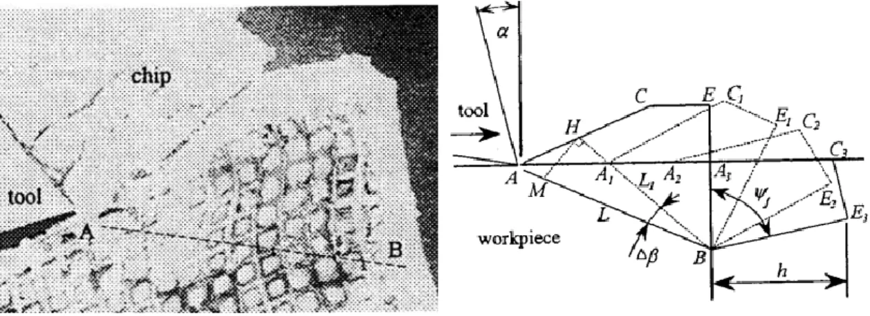
(28) where εa is the shear strain around the cutting tool tip and can be approximated by the von Mises (distortion-energy) theory as 𝜀𝑎 =. 𝛾. , 𝛾 = cot 𝛽0 − cot(𝜙 + 𝛽0 ), and βo is the initial negative. √3. deformation angle and is defined by Eq. (2.15). When the fracture occurs along the negative deformation plane, a negative burr or breakout is formed, leaving a chamfer on the workpiece. It is possible to define the length of the breakout surface η as in Eq. (2.10), from Chern and Dornfeld2). . d a (cot 0.5 cot 0 ) sin ex 1 tan 0 cot ex. (2.10). A positive burr forms in ductile materials. Chern2) was the first researcher to perform a detailed study on the positive burr formation mechanism based on scanning electron microscope (SEM) photographs of the burr formation process during orthogonal cutting, as shown in Fig. 2.8. He assumed that the chip had no effect on the burr formation and would finally separate from the workpiece along the shear plane. In his observations, the process of burr formation was started from initiation state (ACEB) to burr development state (A1C1E1B or A2C2E2B), and finally finished at burr final formed (A3C3E3B), as shown in Fig. 2.8. In addition, the crack started at the tool tip in the primary shear zone, as shown in Fig. 2.9, and changed direction toward the pivoting point. The size of this burr can be defined by its thickness (RBth) and height (RBh), as shown in Eq. (2.11) and Eq. (2.12), respectively.. RBth = w × tanβo. (2.11). RBh = (to + w × tanβo) × sin (θ1 + θ2) × sin θex. (2.12). where w is the initial tool distance from the end of the workpiece and is delineated by Eq. (2.13) and Eq. (2.14) for orthogonal cutting and oblique cutting respectively, as shown by Ko and Dornfeld3). He performed a detailed study on burrs in the oblique cutting process, as shown in Fig. 2.10. θex is the exit angle, to is the undeformed chip thickness, and θ1 and θ2 are the rotation angles near the pivoting point on the burr side and can be defined in Eq. (2.16) and Eq. (2.17).. 14.
(29) Fig. 2.8 SEM microphotograph at initiation state of burr formation2).. Friction zone Primary shear zone. α. xo. Tool. θex. ϕ β0. da Burr. θ2. Negative shear zone. θ1. RBth. Pivoting point Workpiece. w. RBh. Fig. 2.9 Rollover burr that occurs when cutting tool exits workpiece9).. 15.
(30) Ff. cos α cosφ λ α sin φ sin λ cosλ α cosφ α worthogonal σ k0 cos 2 β0 y tan β0 d r 4 2 . (2.13). Ff. cos αc cosφc λ αc cos κ sin φc sin λ cos χ cos λ α c cos φc αc (2.14) woblique σy k0 2 cos β0 tan β0 d r 2 4 d sin β 0 cot φ 0.5 cot β 0 2 3 cot β0 3 cot φ β0 0 dβ 0 cos β 0 sin β 0 cot θ ex . (2.15). θ1 = tan-1(xo / (to + w × tanβo)). (2.16). θ2 = cos-1((w × tanβo × sinθ1) / xo). (2.17). ϕc = tan-1(tanϕ × cosi). (2.18). where λ is the friction angle obtained from λ = tan-1(μ); μ is the coefficient of friction; α is the rake angle in orthogonal cutting; αc is the rake angle in oblique cutting, which is equal to tan-1 (tanα / cosi); dr is the radial depth of cut; 𝑘𝑜 =. 𝜎𝑦 √3. is the shear yield stress. of the workpiece; ϕc is the shear angle in oblique cutting, which can be defined as in Eq.(2.18); cosχ = cosi / cosζ; cosκ = (cosi × sinϕ) / sinϕc; ζ = tan-1(sinα × tani), xo = (0.5 × cotβo) × to; and inclination angle i = π/2 - α.. 16.
(31) Fig. 2.10 Schematic illustration of oblique cutting3).. 17.
(32) 2.3 Parameters that influence burr formation As Gillespie and Blotter1) mentioned in their work, burrs cannot be prevented simply by changing some parameters such as the feed, speed, or tool geometry. To minimize and prevent burrs it is necessary to examine the entire cutting process. The major influences include the workpiece material, tool geometry, tool wear, tool path, and machining parameters. It is not possible to change the workpiece material in some cases, and the tool path is limited, because complex geometries would require burr optimized tool paths that would prolong the cycle time, which would be a negative effect. The burr formation parameters can be reliably separated into direct and indirect factors because of the complex connections and relations between the numerous influencing variables, as shown in Fig. 2.11.. Fig. 2.11 Interdependencies of burr formation parameters7).. 18.
(33) 2.4 Burr measurement Burr measurement methods have been developed by many researchers. Each method has different pros and cons depending on the application conditions, requested measurement accuracy, and burr values to be measured, like the burr height or burr thickness. The types of burr measurement methods can be classified as follows: . One-, two- or three-dimensional. . Destructive or non-destructive. . With or without contact7). Fig. 2.12 Methods of burr detection and measurement7).. 19.
(34) 2.5 Chapter summary This chapter described the general burr formation mechanisms, burr classification, parameters that influence burr formation, and burr measurement methods. The burr definitions based on the work of many researchers, and the burrs from milling operations were described in detail, including about the names and locations of the burrs formed. The mechanics of burr formation and analytical models were discussed from the initial burr state to the final burr formed. Two kinds of workpiece materials were included in this discussion: ductile and brittle materials. Two kinds of burr mechanism models were described in detail: the Poisson burr model and rollover burr model. The many interdependencies of the burr formation parameters were briefly shown to allow a better understanding of the influence of the cutting conditions on burr formation. The burr measurement methods were also shown as basic information on the selection of a method for burr measurement.. 20.
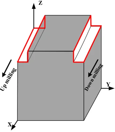
(35) CHAPTER 3. 3. Burr Prediction Method. 3.1 Classification of burrs in end milling In this study, a burr simulation system was developed and used to predict the sizes and locations of burrs. In order to obtain an accurate prediction, burrs were classified based on the relationship between the cutting tool and workpiece in end milling. Two cutting modes were also considered: down milling and up milling, as shown in Fig. 3.1.. Z. Y. X Fig. 3.1 Locations of burrs shown in red for end milling process.. 21.
(36) 3.1.1 Entrance burr This burr is formed on the entrance edge of the workpiece where the cutting tool tips push into it, as shown in Fig. 3.2.. Cutting tool. Cutting tool. Entrance Burr. (a) Up milling. (b) Down milling Fig. 3.2 Entrance burr location.. 3.1.2 Entrance side burr This burr is formed on the entrance side edge of the workpiece where the cutting tool tips push into it, as shown in Fig. 3.3.. Cutting tool. Cutting tool Entrance Side Burr. (a) Up milling. (b) Down milling. Fig. 3.3 Entrance side burr location.. 22.
(37) 3.1.3 Top burr This burr is formed on the top edge of the workpiece where the tool tips push up in the Z direction, as shown in Fig. 3.4.. Cutting tool. Cutting tool Top Burr. (a) Up milling. (b) Down milling. Fig. 3.4 Top burr location.. 3.1.4 Exit burr This burr is formed when the cutting tool leaves the workpiece, as shown in Fig. 3.5.. Cutting tool. Cutting tool Exit Burr. (a) Up milling. (b) Down milling. Fig. 3.5 Exit burr location.. 23.
(38) 3.1.5 Exit side burr This type of burr is formed when the cutting tool leave the workpiece side edge, as shown in Fig. 3.6.. Cutting tool. Cutting tool Exit Side Burr. (a) Up milling. (b) Down milling. Fig. 3.6 Exit side burr location.. 3.2 Application of burr models in end milling 3.2.1 Entrance burr model in up milling The burrs on the workpiece edge shown in Fig. 3.2 (a) occur when the cutting tool moves in the direction to approach workpiece edge. Thus, the Poisson burr model is used to define the burr size. However, tool geometry is also considered in this case for better burr prediction. In Figure. 3.7, the bottom view of the end milling shows a hook shape near the end of the tool tip, which is a critical form to consider. When the blade pushes into workpiece edge, two burr models will apply: rollover burr and Poisson burr models. When the interference point P(Xp, Yp) advances to the center point O(Xo, Yo), the rollover burr model is applied; otherwise, the Poisson burr model is used. This is because, when the point P advances toward the point O, the tool blade motion is seen to push the workpiece material out from the workpiece edge rather than push in. In contrast, when the point O advances toward the point P, the tool blade motion pushes against the side workpiece edge, which is why the Poisson burr model is applied, as shown in Fig. 3.8.. 24.
(39) Fig. 3.7 Bottom view of end milling tool.. Workpiece. Workpiece. Tool motion direction. End Milling Tool. End Milling Tool. P(Xp, Yp). r2 d0. O(Xo, Yo). R r3. θ0. Fig. 3.8 Detail of bottom view of end milling tool in up milling.. 25.
(40) The geometric parameters of the cutting tool can be defined by Eq. (3.1) and Eq. (3.2), where r2 is the hook radius = 1.9 mm and d0 is the hook length of the cutting tool. In this study, we used a cutting tool diameter of 10 mm. Thus, the hook length is 1.65 mm14). r3 is the distance between the tool center and the center of the hook O(Xo, Yo). 2. 2. d d r3 R 0 r22 0 R 2 r22 Rd 0 2 2 2 r 2 d 0 2 2 1 0 tan R d0 2 . (3.1). . (3.2). 3.2.2 Entrance burr model in down milling The cutting tool tip directions are seen to push in at the 1st edge of the workpiece and push out on the 2nd edge of workpiece, as shown in Fig. 3.9. In this case, the Poisson burr model is applied at the 1st edge, and the rollover burr model is applied at the 2nd edge of the workpiece if the point P (Xp, Yp) is advanced toward the point O (Xo, Yo), otherwise the Poisson burr model is applied.. End Milling Tool. Tool motion direction P(Xp, Yp). End Milling Tool. 1st edge O(Xo, Yo). 2nd edge Workpiece. Workpiece. Fig. 3.9 Detail of bottom view of end milling tool in down milling.. 26.
(41) 3.2.3 Entrance side burr model in up milling and down milling In both cases (up milling and down milling), the cutting tool is pushed into the workpiece edge, as shown in Fig. 3.3. Thus, the Poisson burr model is applied in each case.. 3.2.4 Top burr model in up milling and down milling According to Gillespie and Blotter1), the Poisson burr model should be applied for a top burr; however, based on the tool geometry, a modification is needed to increase the accuracy of the burr prediction system. In Figure. 3.10, the red line shows the cutting tool tip blades, which seem to move up because of the helix angle when the tool rotates. For this reason, we assume that the top burr produced is a rollover burr rather than a Poisson burr. Thus, rollover burr models are applied for both down milling and up milling. In addition, the cutting areas in up milling and down milling are different in the case of the top burr view. In down milling, the cutting area is large because the cutting blade is pushed from the outside workpiece edge with a large cutting length and continues to increase the pressure placed on the top edge surface of the workpiece, as shown in Fig. 3.11. In contrast, the cutting areas is small and little pressure on top edge during up milling. The cutting blade starts with a small cutting length and produces less pressure on the top edge, as shown in Fig. 3.12. Thus, the top burr size in down milling will be larger than the top burr size in up milling.. Cutting Tool. Cutting Tool. Cutting Tool. Burr direction. Helix angle. Workpiece. Workpiece. Workpiece. Fig. 3.10 Side view of shoulder end milling9).. 27.
(42) Z. Rotation direction. Y. X. Top burr formed at this red point. Cutting Area. Feedrate. R. Cutting Blade Direction Cutting Blade. Workpiece Top View. Side View. Fig. 3.11 Top burr formed in down milling. Z. Y. Top burr formed at this red point. Workpiece. Cutting removal area. X Lb-a. Feedrate. R. Rotation direction Cutting Blade. Top View. Side View. Fig. 3.12 Top burr formed in up milling.. 3.2.5 Exit burr model in up milling and down milling An exit burr is formed when the cutting tool pushes out from the workpiece edge, as shown in Fig. 3.5. Thus, the rollover burr model is used for both up milling and down milling. In the normal rollover burr model, the depth of the cut is assumed to be small. However, when the depth of the cut is large, a modification of this rollover burr is needed. In the case of a large depth of cut, the cutting blades push the removed volume and generate a plastic deformation zone ABC at a point near where the cutting tool leaves the workpiece edge, as shown in Fig.. 28.
(43) 3.13. The plastic deformation zone ABC was bended around the pivoting point B when the tool was moved forward to the exit surface and the point C was moved to the point D at the final state of a burr development. Thus, the modifications of the burr thickness and burr height can be defined in Eq. (3.3) and Eq. (3.4), respectively.. RBth = w × tanβ0. (3.3). RBh = w × tanϕ / tan β0. (3.4). However, this burr will break because of the ductility of the workpiece material when the equivalent strain at fracture εf ≤ εa is the shear strain. Thus, a shear strain criterion is needed to determine whether this burr is formed. This shear strain can be defined in Eq. (3.5). The equivalent strain at fracture εf can be define in Eq. (2.8), and w, ϕ, and β0 can be defined in Eqs. (2.13) and (2.14), (2.6) and (2.18), and (2.15), respectively.. εa = [(w + RBh) cosϕ – w ] / w. (3.5). Chip α C. Cutting Tool. ϕ A. Workpiece. RBh. β0. w. Burr. D RBth. B. Fig. 3.13 Rollover burr formed when cutting depth is large.. 29.
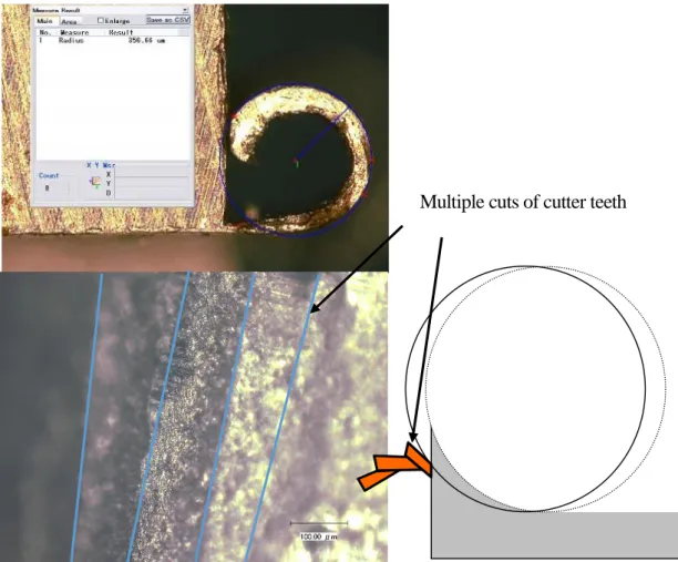
(44) 3.2.6 Exit side burr model in up milling and down milling Exit side burrs are formed, as shown in Fig. 3.6, when the cutting blades push out of the workpiece edge. More than-one cut is required to form these burrs. Based on photo of the surface of a burr, these burrs are formed by multiple cuts of the cutting blades, which turn this burr into a rollover burr, as shown in Fig. 3.14. Thus, the rollover burr model is applied in both up milling and down milling.. Multiple cuts of cutter teeth. Fig. 3.14 Rollover burr formed at side edge by multiple cuts.. 30.
(45) A summary of the burr classifications is given in Table 3.1 and Fig. 3.15. Table 3.1 Classification for use of burr models. Used burr models Burr types Up milling. Down milling. Exit burr. Rollover burr (orthogonal). Poisson burr (orthogonal). Side burr. Rollover burr (oblique). Poisson burr (orthogonal). Top burr. Rollover burr (oblique). Rollover burr (oblique). Entrance burr. Poisson burr (orthogonal). Poisson burr (orthogonal). Entrance side burr. Poisson burr (orthogonal). Poisson burr (orthogonal). Z. Entrance side burr. Exit side burr. Entrance burr. Exit burr Top burr. Exit burr. Exit side burr. Entrance burr. Entrance side burr Rollover burrs. Y. Poisson burrs. X. Fig. 3.15 Locations of burrs in shoulder end milling9).. 3.3 Chapter summary This chapter described the classification of the burrs found in the end milling process. The Poisson burr model and rollover burr model are used for entrance burrs, entrance side burrs, exit burrs, exit side burrs, and top burrs in both up milling and down milling based on their location, tool geometry, and cutting phenomenon . The development of a burr prediction system will be discussed in the next chapter. 31.
(46) CHAPTER 4 4. Development of Burr Prediction System. 4.1 System architecture This chapter presents the development of a burr prediction system for end milling. The proposed approach was implemented in object-oriented software under Windows using C++ Builder13) and the graphical library OpenGL14). The numerical calculation process of the burr prediction system is shown in Fig. 4.1. The input data are from an NC program that was written in the form of G-code and contained in a text file. The system reads information in the text file and uses it in the machining simulator. The burr prediction system, which is called NC simulator, performs with two steps: geometry simulation and physical simulation, as shown in Fig. 4.1. The geometric simulation consists of a geometric model of the workpiece, tool geometry data, and NC data. This simulation is based on a solid modeling system that changes the workpiece geometry with the movement of the tool and removed material. The result of the geometric simulation is the geometric verification of the machined parts; the collision check information about the depth of the cut, width of the cut, and immersion angle; and the reconstruction of the workpiece geometry. Then, the physical simulation is performed using the mechanical and material data of the workpiece, cutting tools, and geometry information provided by the geometric simulation. The physical simulation can instantly estimate the cutting force that will be used to evaluate the burr height and thickness. NC simulator predicts the burr location on a display showing where the burrs were formed and estimates the burr’s size based on each position where the burr models were applied.. 32.
(47) 4.2 Geometric simulation 4.2.1 Z-map model For end milling, a geometric simulation can be achieved as a Boolean subtraction of the tool swept volume model, which represents the space occupied by the cutting tool motion along the tool path, from the workpiece solid model. The Z-map model is used to construct a solid model of the workpiece and cutting tool. During the simulation, NC data containing thousands of tool positions required as many Boolean subtractions results. To verify the simulation results, real-time visualization is also required in the solid modeling system. The Z-map model is the most suitable form for fulfilling these requirements, because the update part model can be made quickly. A frame map is used to display a graphic image.. NC Simulator Y. Workpiece. toi =f sinθi Fri ψ. n θi. Up milling. f. R Feed direction. Down milling. Ω. Fti. X. Geometric simulator. Physical simulator R×ψ. Axial depth of cut. α. to da=(R×θi)/tanα Axial element. ψ:. Lag angle. Fig. 4.1 Numerical calculation process.. This frame is organized as an X-Y matrix of memory locations, and each memory location corresponding to a pixel of the display screen contains the color data to be displayed. The pixel coordinates are represented as (Xi, Yj), where Xi = dx × i, Yj = dy × j, and dx and dy are the pixel or grid sizes (g), as shown in Fig. 4.3, which should be small in order to display a smooth solid model to represent a workpiece. However, this will increase computation time. In addition, i is the index on the X axis, and j is the index on the Y axis, which have relationships with the length of the workpiece on X axis (a) and length of the workpiece in Y axis (b), as. 33.
(48) follow: 0 ≤ i ≤ a/dx and 0 ≤ j ≤ b/dy. The Z-map values are visible on each pixel surface at a specific height. The Boolean subtraction with the Z-map model can simply be performed during the updating of the Z-map height of each pixel point. For example, when the cutting tool moves over a swept volume along the tool path, the Z-map height update will be performed if the stored value is higher than the surface that is swept by the cutting tool at each interference point between the tool and solid workpiece, as shown in Fig. 4.2. The grid size can be freely selected and has a great effect on the accuracy of the cutting conditions, especially the radial depth of cut dr as shown in Fig. 4.3. A small grid size provides better accuracy but increases the computation time. In this study, a grid size g = 0.05 mm was used. The workpiece had a cube shape (a = b = 20 mm) with height Wh = 30 mm and cutting tool rake angle α = 30o.. Cutting tool Z Z-map height initial. Depth of cut. Workpiece. Z-map height update X. Z-map height update = Z-map height initial – Depth of cut. Fig. 4.2 Boolean subtraction with Z-map model.. 34.
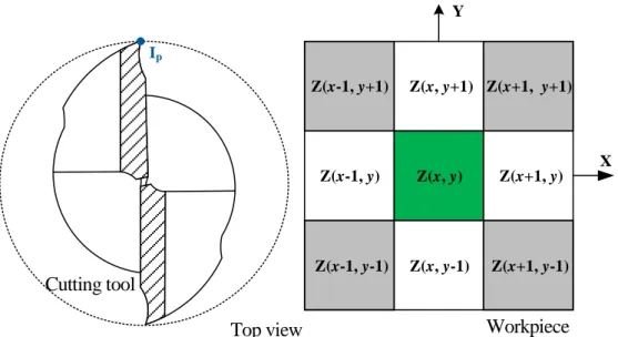
(49) Grid center points by 2D arrays of Z-map. g. Workpiece (top view). (X+1, Y+1) (X+1, Y) (X+1, Y-1). Vector tool feed direction (X, Y+1). (X, Y). (X, Y-1). (X-1, Y+1). (X-1, Y). (X-1, Y-1). P(Xp,Yp). O(Xo,Yo) Up Milling. Vector tool feed direction. Down Milling. Hook. Feed rate. Rotation Direction. dr (up milling). dr (down milling). X Y. Fig. 4.3 Z-map model used to represent workpiece9).. 35.
(50) 4.2.2 NC program analysis model The analysis model was developed to read and store the information from the G-code syntax. This analysis model can recognize the G-code syntax such as the G function, M function, and coordinate letters X, Y, Z, along with the cutting condition. This G-code or NC program provides the command information for the NC machine to move base on the input code. In this study, the NC program analysis model had the ability to translate the NC code and send information to the geometric simulator to execute the simulation process display. The G-code functions that the NC program analysis model can recognize are listed in Table 4.1.. Table 4.1 G-code functions15). Code Functions. Description Move fast forward to the specified coordinates from. G00. Fast forward. G01. Linear interpolation. G02. Circular interpolation. the current position. Move in a straight line at the specified feed rate to the specified coordinates from the current position. Move in the clockwise direction with the specified feed rate to the specified coordinates. Move in the counterclockwise direction with the. G03. Circular interpolation. M00. Compulsory program stop. Stop the execution of the program.. M03. Spindle rotation normal. Rotate the spindle in the clockwise direction.. M30. Program end. specified feed rate to the specified coordinates.. Represents the end of the program. It is always used with reset and rewind.. 36.
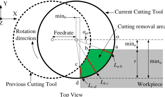
(51) The NC code is written in text file (.txt) and included in the program folder. The NC program analysis model read the information contained in that text file. The flow of the program execution can be described as follows:. 1. Create a two-dimensional matrix array to store the G code information, 2. Read a line of code in the text file and store it in the matrix, 3. Copy that information and update the information for the next line to use, 4. Read the next line and save it in the matrix, and 5. Repeat steps 3 and 4 until finished with the code in the text file.. 4.3 Physical simulation In the physical simulation, the cutting force at a certain instance is calculated using a force model. This force model is based on the axial depth of cut, cutting areas, and cutting constant. In this study, three patterns for the cutting process simulation are discussed for force model development, including the entrance pattern, ready pattern, and exit pattern of the cutting tool from the workpiece. These patterns were applied for both up milling and down milling.. 4.3.1 Cutting length calculation (1) Entrance pattern In this pattern, the cutting tool starts to approach the workpiece edge as shown in Fig. 4.4. The cutting lengths vary between points a and b, b and c, and c and d, as represented by La-b, Lb-c, and Lc-d, respectively and can be defined by Eq. (4.1) to Eq. (4.3), respectively. Lab R . min a sin a. Lbc R f cos b R 2 f 2 sin 2 b. Lcd R . min b cos c. (4.1). (4.2). (4.3). 37.
(52) Y. X. Current Cutting Tool. minb. Z Rotation direction. Cutting removal area. αai. Feedrate. o a. b c d. Previous Cutting Tool. La-b. Lc-d. Lb-c. mina r. maxa. Workpiece. Top View Fig. 4.4 Cutting length in each segment at entrance pattern of cutting tool. where R is the cutting tool radius; f is feed rate; and αa, αb, and αc can be found using Eq. (4.4) to Eq. (4.6), respectively. min a R . (4.4). min a R 2 min a 2 f . (4.5). a sin 1 . b tan1. . R 2 f min b 2 c tan min b 1. . . (4.6). (2) Ready pattern In this pattern, the cutting tool fully engages the workpiece, as shown in Fig. 4.5. Two cutting lengths vary, in the segments from point a to b and b to c (La-b and Lb-c), which can be defined in Eq. (4.7) and Eq. (4.8), respectively.. 38.
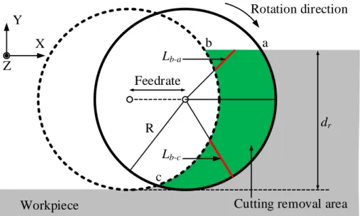
Gambar
+7


Dokumen terkait
Berdasarkan konsep dasar di atas salah satu paradigma penting yang ditawar- kan oleh manajemen risiko di dalam mengelola risiko adalah bahwa risiko dapat didekati dengan
Berdasarkan hasil penelitian disimpulkan bahwa terjadi peningkatan writing skills peserta didik melalui penerapan model Problem Based Learning pada materi Sistem
Penelitian ini bertujuan untuk mengetahui gambaran obat diabetes melitus pada pasien DM geriatri di Instalasi Rawat Inap RS X Klaten tahun 2011 dan mengetahui ketepatan
Segala puji syukur kehadirat Tuhan YME yang telah melimpahkan seluruh rahmat serta karunia-Nya sehingga penulis diberikan kelancaran dan kemudahan dan mampu menyelesaikan
This paper aims to investigate the c ommon strategies that are used by the teachers in dealing with students’ silence at the seventh grade in English classrooms..
Menimbang, bahwa berdasarkan pertimbangan tersebut di atas, Majelis Hakim berpendapat eksepsi Tergugat beralasan sehingga harus dikabulkan dengan demikian Pengadilan
Kepada Penyedia Jasa Pengadaan Barang/Jasa yang mengikuti lelang paket pekerjaan tersebut di atas dan berkeberatan atas Pengumuman ini, diberikan kesempatan mengajukan
Maka perlu dilakukan perbaikan secara terus-menerus untuk meningkatkan pengaruh Program Booking service terhadap kepuasan Konsumen, Keluhan yang banyak dihadapi oleh
