Aerodynamics of Wind Turbines - Martin OL Hansen

FSC (the Forest Stewardship Council) is an international network to promote responsible management of the world's forests. The intention is by no means to provide a complete historical overview of wind turbines, but merely to highlight some important milestones in their development and to provide examples of the historical exploitation of wind energy.

4.1 Illustration of the streamlines past the rotor and the axial

Short Historical Review

Before addressing more technical aspects of wind turbine technology, an attempt is made to give a brief general introduction to wind energy. Large non-commercial prototypes were built to evaluate the economics of wind-generated electricity and to measure loads on large wind turbines.

Why Use Wind Power?

Since the oil crisis, commercial wind turbines have gradually become an important industry with annual turnover in the 1990s of more than US$1 billion per year. In addition, noise and visual impact will be less important in the future as more wind turbines are placed offshore.

The Wind Resource

The explanation lies in the way the boundary layer separates from the top of the airfoil. It is known from the viscous boundary layer theory (see e.g. White, 1991) that the pressure is approximately constant from the surface to the edge of the boundary layer, i.e.

Figure 1.1 Horizontal-axis wind turbine (HAWT)

The vortices on the wing (bound vortices) model the lift, and the trailing vortices (free vortices) model the vortex sheet, which originates from the three-dimensionality of the wing. At the wingtips, the induced velocity attains a value which exactly ensures zero lift.

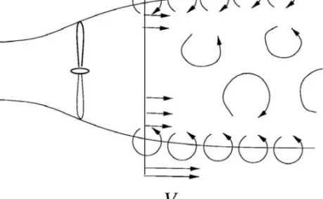
Figure 3.1 Streamlines flowing over and under a wing

Vortex System behind a Wind Turbine

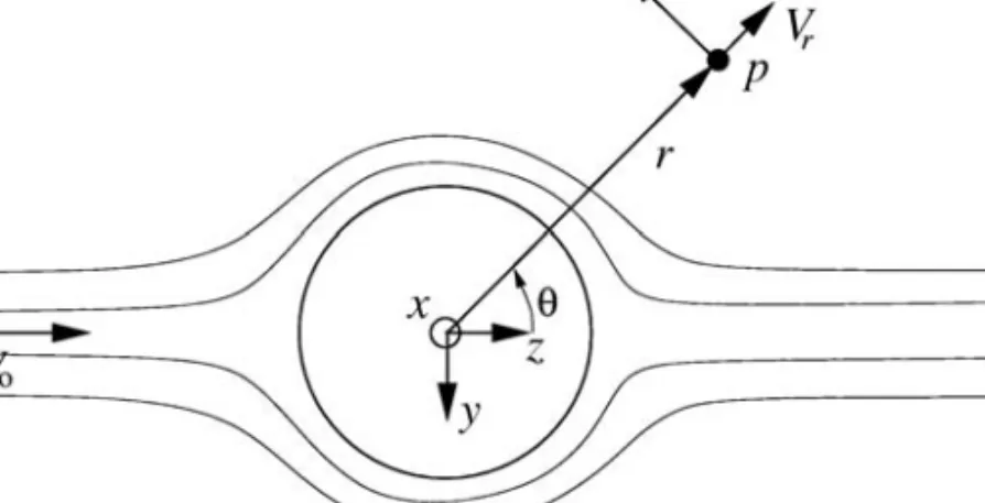
Furthermore, on the lateral boundary of the control volume shown in Figure 4.2, the force of the pressure has no axial component. It is seen that the velocity in the rotor plane is the average of the wind speed Vo.

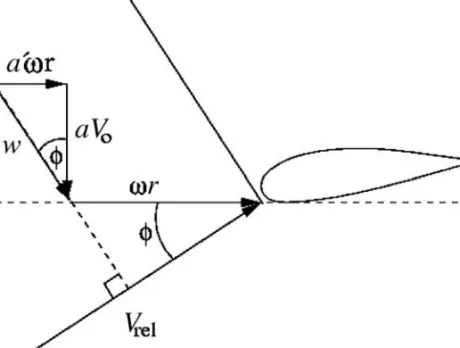
Figure 3.8 Rotor of a three-bladed wind turbine with rotor radius R

Effects of Rotation

It can be seen from equation (4.26) that for a given power Pand wind speed, the component of the azimuthal velocity in the track Cθ decreases with increasing rotational speed ω of the rotor. In 1-D torque theory, the actual geometry of the rotor—the number of blades, the twist and chord distribution, and the airfoils used—is not considered.

Figure 4.8 The velocity triangle for a section of the rotor

Prandtl’s Tip Loss Factor

Bis the number of blades, Ris the total radius of the rotor, ris the local radius and φ is the flow angle. Deriving Prandtl's tip loss factor is very complicated and is not shown here, but a full description can be found in Glauert (1935).

Glauert Correction for High Values of a

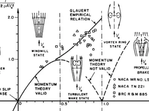
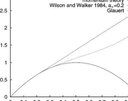
In Figure 6.5, the two expressions for CT(a) are plotted for F = 1 and compared with simple momentum theory. In order to correctly calculate the induced velocities for low wind speeds, equations (6.44) and (6.42) must be substituted for equation (6.35) from simple momentum theory.

Figure 6.5 Different expressions for the thrust coefficient C T versus the axial induction factor a

Annual Energy Production

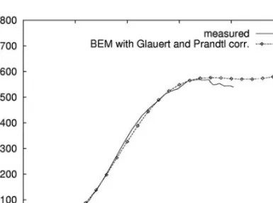
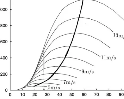
The power curve was measured (Paulsen, 1995) and the comparison between the calculated and measured power curve is shown in Figure 6.7 to give an idea of the accuracy of the BEM model. The advantage of plotting the power factor as a function of the inverse tip speed ratio is that λ-1 increases linearly with the wind speed Vo.

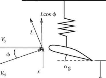
Stall Regulation

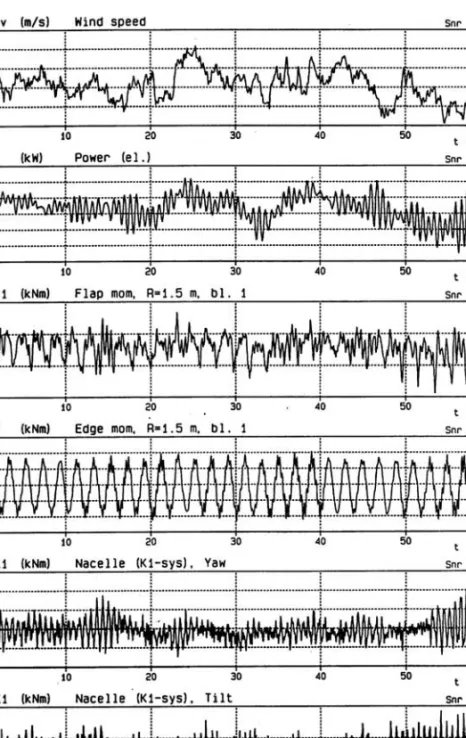
The first curve in Figure 7.3 shows the wind speed at hub height, the second curve shows the generator rotation speed n and the last curve shows the corresponding power as a function of time. The calculated mechanical power curves for the NTK 500/41 wind turbine operating as a stall and pitch wind turbine are shown in Figure 7.10.

Figure 7.1 Atypical torque characteristic for an asynchronous generator

Yaw Control

However, due to the turbulent properties of the wind, the power curve on a true pitch-controlled machine is not as steep near Pnomas, as the theoretical curve indicates in Figure 7.10, so the increase in annual production is probably slightly lower than estimated at basis of the theoretical power curves.

Variable Speed

It is possible to analytically calculate the geometry of design 1 in Figure 8.1 with the already derived equations as described in, for example, Glauert (1935). Note that the cone angle must be negative for the blades to cone as shown in figure 9.1.

Dynamic Wake Model

Further, it is noted that the equations must be solved iteratively since the flow angle and thus the angle of attack depend on the induced velocity itself. This can be done since the induced velocity changes relatively slowly in time due to the dynamic wake pattern.

Dynamic Stall

Cl,invis usually an extrapolation of the static aerofoil data in the linear region; a way to estimate Cl,fsand fsstis shown in Hansen et al (2004). It is seen that the mean slope of the lift curve, dCl/d, becomes positive for the dynamic aerofoil data in stall, which is beneficial for stability.

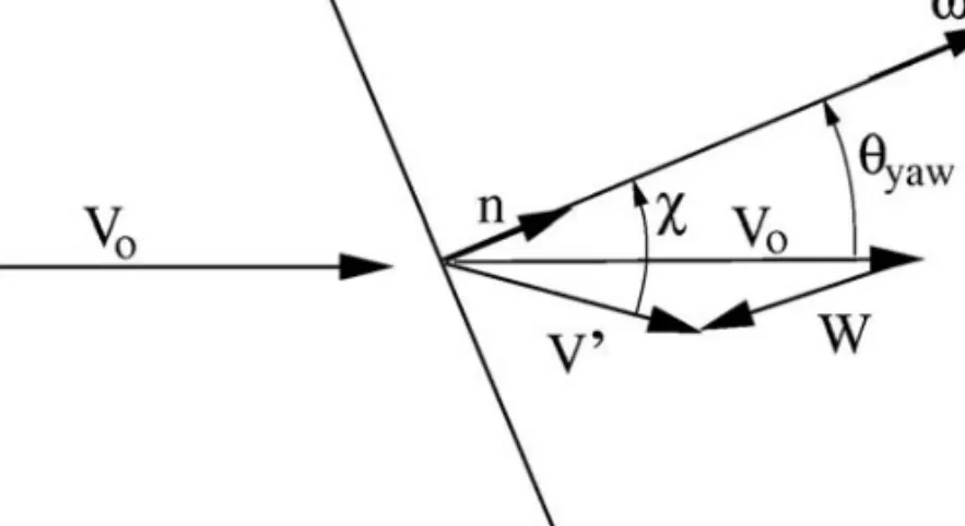
Yaw/Tilt Model

It can thus be seen as a model of the time it takes for the viscous boundary layer to evolve from one state to another. Thus, the angle of attack can be evaluated using equation (9.10) and the lift, drag, and moment coefficients can be looked up in a table.

Figure 9.10 Yawed rotor disc in wind field

Deterministic Model for Wind

A simple model for the influence of the tower is to assume potential flow (see Figure 9.12). Furthermore, the turbulent part of the real atmospheric wind should be added for a realistic time simulation of a wind turbine. 1976) Helicopter Dynamics, Edward Arnold Ltd, London.

Description of Main Loads

A negative mold is made for the upper part (suction side) and the lower part (pressure side) of the blade. It is seen that the thick layer of mats and epoxy in the middle of the skin and the lanes form a box-like structure.

Figure 10.2 Example of computed loads using FLEX4 for a mean wind speed of 11m/s

Deflections and Bending Moments

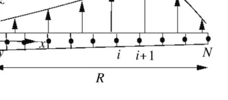
All other things being equal, the first major axis can be assumed to lie along the chord line, which is only true for a symmetrical airfoil. If the loads are given at discrete points, as shown in Figure 11.9, and the loads are assumed to vary linearly between two points i and i1, then equations (11.11) to (11.14) and equations (11.21) to (11.24) can be are integrated to give the following numerical algorithm to calculate bending moments and deflections.

Numerical Algorithm for Determining the Bending Moments and Deflection

The boundary conditions are for a cantilever beam and the inertia terms in equations (11.11) and (11.12) are neglected for simplicity, but must be added for an unsteady calculation.

A Method to Estimate the First Flapwise, First Edgewise and Second Flapwise Eigenmodes

The shape of the deflection, uz1f and uy1f, of the first eigenmode of the flap is now known, as sketched in Figure 11.10. After a few iterations, the deflection shape of the first edge eigenmode, node and uyle, is known, as shown in Figure 11.11.

Figure 11.10 First flapwise eigenmode (1f)

Principle of Virtual Work and Use of Modal Shape Functions

The values in the vector x that describe the deformation of the structure, xi, are known as general coordinates. The elements in the mass, stiffness, and damping matrix depend on the system, and in the case of a federated system, also on the discretization.

SDOF

Aerodynamic Damping

The first column is the generalized force required to obtain a unit velocity of the first generalized coordinate, i.e. the first column in the stiffness matrix can be found using the generalized force required to obtain a unit static displacement of the to obtain first generalized coordinate, i.e.

FEM Models

For example, when the method is used on a complete wind turbine structure, the equation of motion becomes fully coupled. This book does not attempt to use the FEM approach for modeling a wind turbine, but more details and further reference can be found, for example, in Hansen et al (2006). 2005) 'Aeroelastic simulation of wind turbine dynamics', PhD thesis in Structural Mechanics, Royal Institute of Technology, KTH, Stockholm, Sweden Hansen, M. State of the art in aerodynamics and aeroelasticity of wind turbines', Progress in Aerospace Sciences, vol 42 , no 4, pp FLEX4 simulation of wind turbine dynamics' in Proceedings of 28th IEA Meeting of Experts Concerning State of the Art of Aeroelastic Codes for Wind Turbine Calculations (available through the International Energy Agency). 2002) 'Verification of European design codes for wind turbines, VEWTDC;.

Gravitational Loading

This load is easily recognized in Fig. 10.2 in the time series of the edge bending moment. Since a wind turbine blade can weigh several tons and be more than 30 m long, stresses due to gravity loading are very important in fatigue analysis.

Inertial Loading

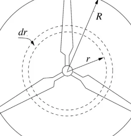
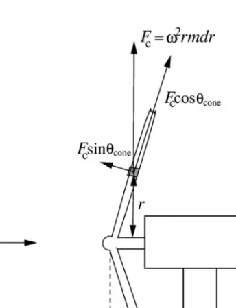
The centrifugal force acting on the rising part of the blade at a radius r from the axis of rotation as shown in Figure 13.3 is Fc = ω2rmdr, where Mis is the mass of the rising part and ω is the angular velocity of the rotor. Because of the taper, the centrifugal force has a component in the blade-wide direction, Fccosθcone, and a component normal to the blade, Fcsinθcone, as shown in Figure 13.3.

Aerodynamic Loading

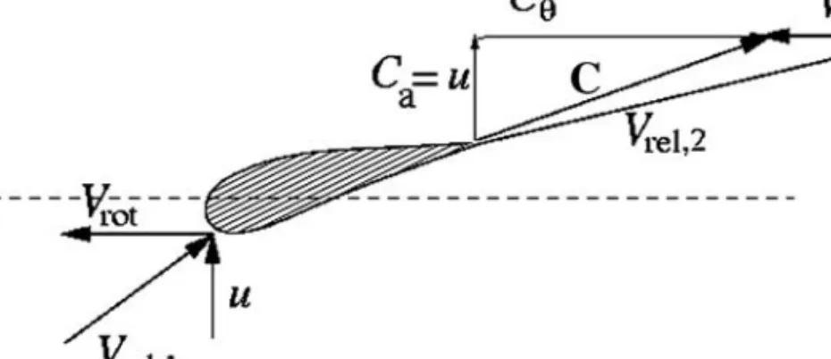
Wind shear produces a sinusoidal variation of the wind speed seen by a blade with a frequency corresponding to the rotation of the rotor 1P. Therefore, both the relative speed seen by the blade and the angle of attack vary with the frequency of the rotor, ω.

Table 13.1 Roughness length table z o [m] Terrain surface characteristics

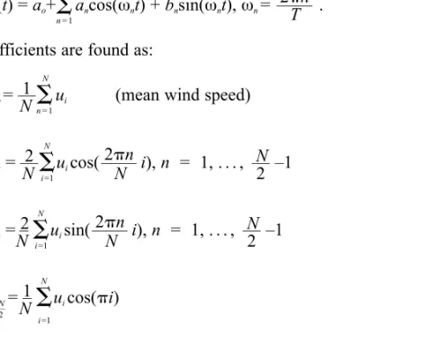
Wind Simulation at One Point in Space

The phase angle ϕ is not reflected in the PSD function and can be modeled using a random number generator that produces a value between 0 and 2π. Using equation (14.14) it is very easy to calculate a discrete time series with exactly the prescribed PSD function.

Figure 14.1 shows that the highest frequency that can be resolved is f h = f s / 2

3-D Wind Simulation

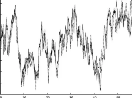
It should be mentioned that the time history of the wind seen through a point on the blade is different from the time history of a point fixed in space. The turbulence intensity, I, is defined as σ/V10min, where σ is the standard deviation of the wind speed within the 10 minute time series.

Figure 14.3 Computed time series of wind speed in two points separated by 1m

Appendix A

Bernoulli's equation requires that the flow be stationary, that no external forces are present, and that the flow be incompressible and frictionless. Bernoulli's equation is generally valid along the flow, but if the flow is without rotation, the equation is valid between any two points.

Appendix B

V2s time average wind speed over a period of 2 seconds v angle between chord line and first major axis v y component of velocity vector. Wy tangential component of induced velocity Wz normal component of induced velocity q2s dynamic pressure based on V2s.

Greek Characters