by OF

EXTREME VALUE ANALYSIS O F FLUCTUATING AIR LOADS ACTING ON A CYLINDER

T h e s i s by J a y Chung Chen

In P a r t i a l Fulfillment of the R e q u i r e m e n t s F o r t h e D e g r e e s f

Aeronautical Engineer

California Institute of Technology P a s a d e n a , California

a

⁹⁶⁷

(Submitted September 2 3 , '1 966)

ACKNOWLEDGMENT

The author would like to express his appreciation to Dr. Y. C.

Fung for his encouragement and guidance for this study, and to the National Science Foundation for providing financial assistance. A

s i n c e r e thanks is given to D r . L. V. Schmidt, Mr. R. E. Spitzer and Mr. M. E. J e s s e y for thei'r very helpful advice and assistance f o r data handling.

-

^{i i i}

-

ABSTRACT

The fluctuating a i r loads over the surface of a smooth, cantilevered c i r c u l a r cylinder perpendicular to a flow in the supercritical Reynolds number ranging f r o m 2 . 5 ~ 1 0 ~ to 7 . 5 ~ 1 0 5 have been investigated according to Gumbel's e x t r e m e value

theory

.

The envelope of the extreme values of the p r e s s u r e was found to be much g r e a t e r than the static p r e s s u r e and the root- mean- square value s and decreased with increasing Reynolds number.

On the other hand, the envelope of the e x t r e m e values of the resultant f o r c e was generally unrelated with ReynoPds number.

NOMENCLATURE Symbols

F(x)

Definition

Probability function that the value of variate is l e s s than a c e r t a i n x .

Density of the probability function.

Probability that the l a r g e s t value faus s h o r t of x

,.

Number of independent observations.

Reduced extreme value.

The mean of a probability distribution.

The standard deviation of a probability distribution.

P a r a m e t e r s . E u l e r ' ^s constant.

Return period.

C ons tant s

.

Number s f batche s s f data.

Reynolds number.

Lift coefficient Drag coefficient

Coefficient s f resultant force.

Dynamic p r e s s u r e .

T A B L E O F CONTENTS

T I T L E PAGE

INTRODUCTION 1

THE E X T R E M E VALUE THEORY 2

APPLICATION TO THE FLUCTUATING AIR LOAD 5

ACTING ON A CYLINDER

ENVELOPE O F EXTREME VALUES O F PRESSURE 9 ENVELOPE O F EXTREME VALUES O F RESULTANT 12 F O R C E

VARIATION O F THE EXTREME VALUE INTERVAL 1 3

DISCUSSION 1 4

CONCLUSIONS R E F E R E N C E S

WORKSHEETS 1 7

TABLES 20

FIGURES 22

ILLUSTRATIONS FIGURE

Probability Pape r

Extreme Value Envelope of P r e s s u r e Coefficient a t Re = 2 . 5 ~ 1 0 ~

E x t r e m e Value Envelope of P r e s s u r e coefficient a t Re = 3 . 8 ~ 1 0 5

Extreme Value Envelope of P r e s s u r e Coefficient a t Re = 5 . 3 ~ 1 0 ~

Extreme Value Envelope s f P r e s s u r e Coefficient at We = 6 . 5 ~ 1 0 ~

E x t r e m e Value Envelope of P r e s s u r e Coefficient a t Re = 7 . 5 ~ 1 0 ~

Extreme Value of Resultant F o r c e Extreme Value v s . Intervals

Initial Distribution

PAGE 2 2 23

- 1

-

1 . INTRODUCTION

The knowledge of fluctuating a i r loads f o r flow over a c i r c u l a r cylinder in the s u p e r c r i t i c a l regions h a s engineering application to c u r r e n t problems of importance in dealing with the response of l a r g e cylindrical objects such a s smokestacks and m i s s i l e s on open launch pads. Many investigations have been made (Refs

.

^l

,

^{2, 3 , 41, and}

one important nature of the a i r Boads that was shown i n every inves- tigation is the randomness of a i r Boads a t s u p e r c r i t i c a l flow region.

F o r the problem of s t r u c t u r a l design based on ultimate static f a i l u r e , the l a r g e r air loads a r e of particular i n t e r e s t , a s they a r e likely t o cause s t r u c t u r a l damage. As i t will be shown l a t e r , the

e x t r e m e a i r loads a r e much g r e a t e r than the average loads. The designer would like to know how l a r g e these e x t r e m e a i r loads a r e and how often they occur. Because the l a r g e r a i r loads a r e infre- quent, m e a s u r e m e n t s available f r o m limited s a m p l e s of data will generally not extend to the l a r g e r and c r i t i c a l values of a i r loads.

Consequently

,

a n important problem in these investigations is the development of techniques f o r estimating the probabilitie s of en- countering these l a r g e r value s ,

The s t a t i s t i c a l theory of e x t r e m e values which w a s developed by E. J. Gumbe1 h a s indicated a rational approach t o the problem of predicting the probability of occurrence of e x t r e m e values.

Throughout t h i s r e p o r t , this theory is applied.

l e s s than a c e r t a i n x , and let f(x) = F' (x) be the density of probability, henceforth called the initial distribution. Then the probability that n independent observations a l l fall s h o r t of x is evidently ~ ~ ( x ) , by the r u l e s of multiplication of independent combined events. In other words, this is the probability for x t o be the l a r g e s t air load among n independent observations. L e t x

=

xn, then

We c a l l @ the probability of e x t r e m e values, and consider

which is a new probability distribution.

F o r some given initial distribution F ( x ) , @(x) can be solved explicitly. F o r example (Ref. 5), if

is a normal distribution, where m is the mean and cr is the standard deviation, then

where

and

But in the practical c a s e s , either the initial distribution is unknown o r it is too difficult to obtain. Gumbel h a s shown that if the initial distribution belongs to the so -called exponential type, then the asymptotic form of the extreme value distribution (Ref. 6 ) i s given by eqs. (4) and (5). The p a r a m e t e r s a and m can be e s t i - mated from the limited samples of the extreme value observations, i . e . ,

Here m and ^(B a r e , respectively, the mean and standard deviation of the sample of extreme value observations.

F u r t h e r m o r e , Gumbe% constructed a "probability paper"

om which the extreme values of the a i r load obtained from N batches of data, each consisting of n observations a r e t r a c e d along the ordi- nate. The probability @ (x) and y a r e traced along the a b s c i s s a .

'khe number of return period T(x) defined by

can be plotted along another scale parallel to G(x). Since i n p r a c - tical c a s e s the number s f e x t r e m e observations N is not infinity, the modification was made a s follows.

P ( N )

u = m

- -

_{a! *} ^Lim

Y(N)

^y

N-a3

where cr(N) and

Y(N)

a r e functions of N which was tabulated in Ref, 6 .

The detailed summary of the theory can be found i n Ref. 7.

3 . APPLICATION OF THE FLUCTUATING AIR LOAD ACTING ON A CYLINDER

The experimental data on the fluctuating a i r load acting on a cylinder were taken f r o m a t h e s i s which was done by Robert E.

Spitzer, (Ref. 4).

The experiment was mainly the recording of the fluctuating p r e s s u r e and resultant f o r c e s from a smooth cylinder (8.54-inch d i a m e t e r ) cantilevered 8 . 1 d i a m e t e r s from a flat floor in the wind

5 5

tunnel. The range of Reynolds number was 2.5~110 <Re<il. 5x1 0

.

F1uctuating p r e s s u r e s w e r e m e a s u r e d through a 0.025-inch orifice by a reluctance -type p r e s s u r e t r a n s d u c e r . The angular

position was determined by rotation of the model to align the orifices with a p r o t r a c t o r to within one degree of the d e s i r e d value. P r o p e r back p r e s s u r e was supplied to the transducer by a second orifice placed 0.75-inch below the transducer orifice a t the same angular position. To obtain a steady back p r e s s u r e , a calibrated 'sdashpot"

was placed in the system to dampen the fluctuations in p r e s s u r e f r o m the back p r e s s u r e orifice, and this s t a t i c surface p r e s s u r e was m e a s u r e d using a fluid-in-glass manometer.

Lift fluctuations w e r e m e a s u r e d using the instrumented sections built by Schmidt. Lift was determined by 18 p r e s s u r e t r a n s d u c e r s , nine on each side of the section, spaced to cover equal portions s f the cylinder chord. E l e c t r i c a l integration of each nine gave the loading on each side of the cylinder. A differential

B 08 kc c a r r i e r amplifier gave the amplified e l e c t r i c a l difference between the two s i d e s , i. e

. ,

fluctuating lift signal.

The original data were recorded on the magnetic tape.

Because a tremendous amount of data has to b e handled, the

records were converted to the digital form by using the Biological System Mark

II

Analog

-

Digital converter at Caltech Computing Center. The signal of the analog tape was sampled and converted to a binary number a t a pre-selected timing r a t e , 500 samples per second, whereupon i t i s transferred to a digital tape via an input sub-channel in the IBM 7094 system; then a program was made according to the theory, to select the extreme values.

At each angular orientation of the cylinder in the flow and at a specific Reynolds number, the experiment has about 3 minutes of data in analogy form. The Analog-Digital converter converts them into the digital form by the r a t e of 500 samples per second: -

in other words, each experiment has 90,000 samples which a r e the input data of the computer program. The program was made to scan the input data and pick up the l a r g e s t value among each 2588 samples in sequence. In other words, the extreme values a r e selected at each 5 second interval (2500 samples in digital form). Totally, about 36 extreme values a r e obtained for 3 minutes s f data for every experiment. They a r e not necessarily the f i r s t 36 largest data among 98,000 samples, but they a r e the largest among the each 2500 samples a s ~ e q u i r e d by the theory.

The time interval between each successive extreme values i s also not necessarily 5 seconds, it can be any value between zero

seconds and P O seconds.

In worksheets 1 and 2, a n example of lift coefficient ( r e s u l - tant f o r c e in the direction perpendicular to a i r flow) a t Reynolds number 7 . 5 ~ 1 0 5

,

i s given. Those e x t r e m e values x a r e picked up f r o m the input data by the computer a t 5 second intervals. These e x t r e m e values a r e a r r a n g e d according to t h e i r magnitude in work- sheet 1

.

Then the ordering number, A, ( h e r e called the cumulative frequency) i s a s signed. The plotting position i s then computed

simply a s A./(N+~), IN being the number of batches of data. (Notice that t h e r e a r e only 35 e x t r e m e values instead of 36; the l a s t one in the digital tape was ruled out due to electronic noise.) Then the mean m and the standard deviation r a r e calculated f r o m the data according to worksheet 2. The p a r a m e t e r s a and u can be estimated according to Ref, 6 , a s shown i n sheet 2. Figure l shows Gumbel's probability paper. The experimental data f r o m worksheet P a r e plotted with the plotting position X/N+P as a b s c i s s a and the corresponding x a s ordinate. The theoretically extimated straight line relationship of the e x t r e m e distribution is calculated in work- sheet 2 and plotted i n F i g . 1

.

The control c u r v e s , which r e p r e s e n t 95% confidence level, a r e a l s o plotted. The method of calculating such control c u r v e s i s explained in detail in Ref. 6 and the r e s u l t s a r e shown in sheet 2 .

In Tables 1 and 2 , the p a r a m e t e r s Q! and ra a r e l i s t e d f o r C the p r e s s u r e coefficient, and Cf, the coefficient of resultant

P

f o r c e , f o r different Reynolds numbers and different angular o r i e n - tations. (8 = 0 corresponds t o the flow direction.

1

It is c l e a r now, by specifying the extreme value of the p r e s s u r e o r the force which can be withstood safely by the cyl- inder, one can calculate the probability of occurrence of that extreme value by means of eqs. (4) and (5). Then the length of the time interval in which such an extreme value i s expected to occur once, multiplying the r e t u r n period from eq. (1 0) with the time interval of observation, (e. g.

,

5 seconds in this c a s e ) . Conversely, by specifying the lift of the structure, one can obtain the l a r g e s t air load that will be encountered within this period.

- 9 -

4. E N V E L O P E O F E X T R E M E V A L U E S O F P R E S S U R E

If we specify the period that the cylinder will be exposed to the a i r flow to be 500 seconds, then the r e t u r n period, T(x), a t 5-second intervals will be 100. In other w o r d s , the probability

@(x) i s , by eq. (101,

The reduced extreme value y can be obtained by eq. (4):

And then the l a r g e s t value of the air load which the cylinder will encounter within 580 seconds can be obtained by eq. (5):

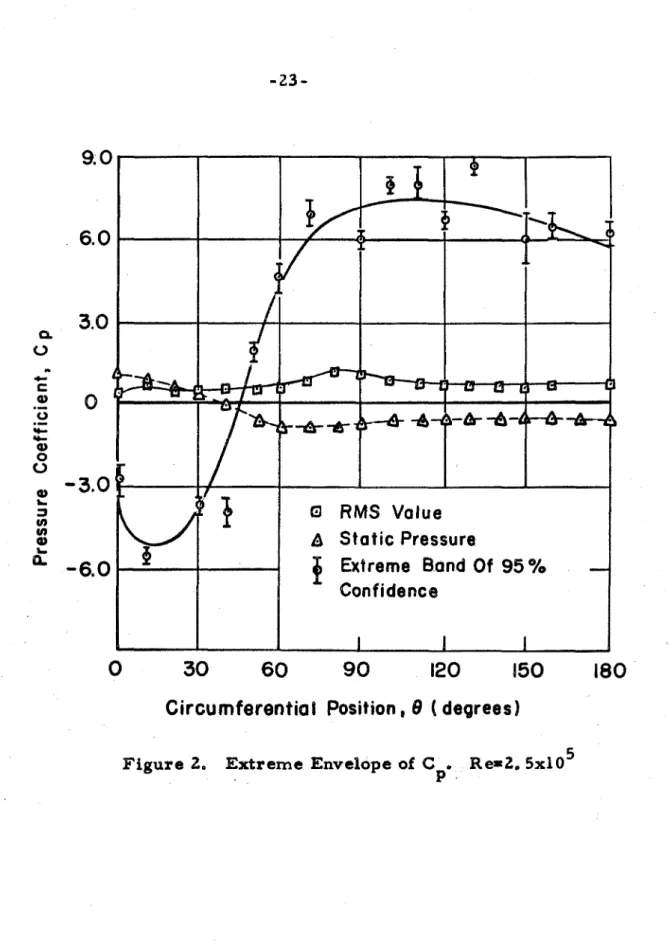
In F i g u r e s 2 , 3 , 4, 5, and 6 , these l a r g e s t p r e s s u r e coefficients within 500 seconds w e r e plotted f o r different Rey- nolds numbers and angular orientations.

It i s n e c e s s a r y to emphasize that the e x t r e m e value curve did not r e p r e s e n t any particular loading. They a r e the m o s t prob- able values of a i r Bsad the cylinder will encounter within 500 seconds.

Therefore, the curve f o r m s a n envelope from which the l a r g e s t expected value can be obtained. Clearly, this kind of information is of vital importance to the s t r u c t u r e designer.

Now l e t u s look a t each figure individually.

Hn

Figure 2 , Re = 2 . 5 ~ 1 0 5

.

^The

C

with the l a r g e s t absolute value i s negative

P

f r o m 8 =

o0

(parallel to f r e e s t r e a m ) to 8 40 and then becomes 0

positive. The maximum C 8.0 occurs approximately a t €I=

loo0.

P

Since the Reynolds number i s not v e r y high, a periodic s t r u c t u r e i n the p r e s s u r e history was observed during the digitization through a n oscilloscope. However, the signals w e r e somewhat random.

The C ' s a r e plotted with 95% confidence band. The extreme P

envelope i s defined by a curve which t r a c e s along these C ' s . P

Also the static p r e s s u r e s , which were m e a s u r e d by a fluid-in-glass manometer connected with a n orifice on the cylinder surface, a r e plotted. The root-mean-square values of p r e s s u r e , which w e r e recorded by a Ballantine type 320 T r u e RMS Voltmeter with capaci- tive damping to give a long time constant, a r e a l s o plotted f o r com- parison. The envelope shown in this picture cannot be predicted by only knowing the p r e s s u r e i s periodic.

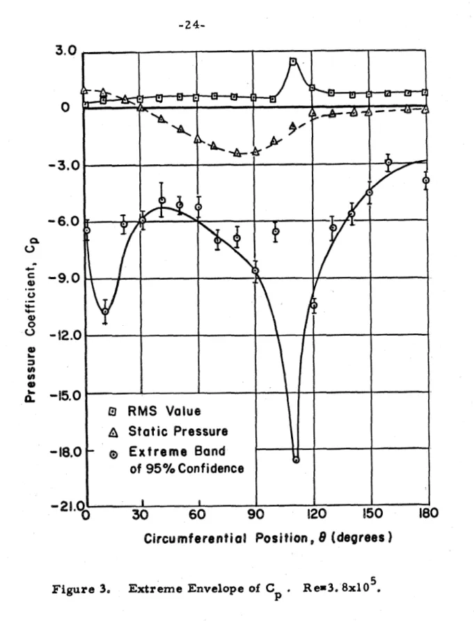
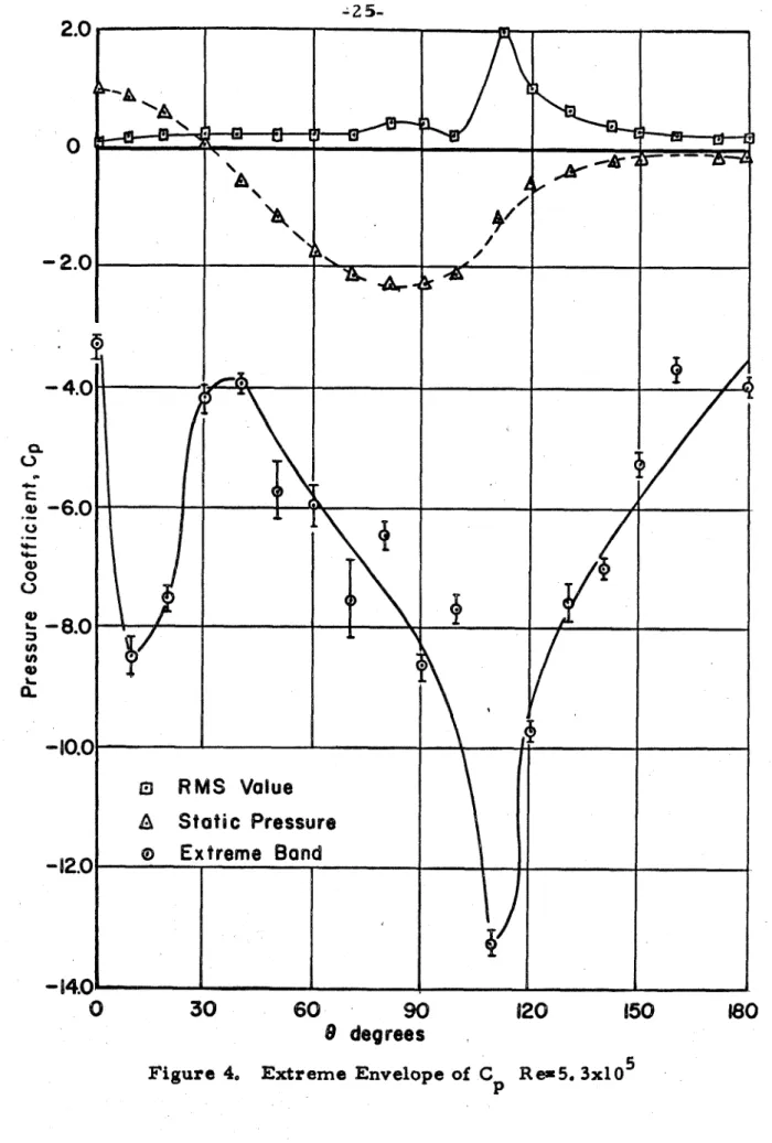
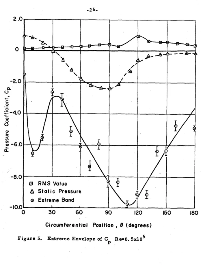
F i g u r e s 3 , 4, and 5 a r e f o r Reynolds number 3 . 8 ~ 1 0 5

5 5

5 . 3 ~ 1 0 and 6 . 5 ~ 1 0

,

respectively. One can s e e t h e r e a r e two peaks in each e x t r e m e value envelope. One is a t 8 = 1

o0

which i s the s m a l l e r one, the other i s a t 8 = POO", which is the maximum extreme value. Comparing these two peaks with static p r e s s u r e which is also plotted by dotted lines, i t s e e m s that t h e r e i s a phase shift, since the two l a r g e s t static C ' s a r e a t 8 =

o0

and

P

8 = 8 0 ~ . Two phenomena a r e observed: one i s that all extreme values a r e negative. The other i s that the peak values a r e de

-

creasing with increasing Reynolds number. ]Em sther words, that the l a r g e s t p r e s s u r e i s not n e c e s s a r y happened f o r the l a r g e s t

W

eynolds number.

-11-

Once again if we compare the extreme value envelope with the static p r e s s u r e , the f o r m e r i s considerably g r e a t e r than the l a t t e r

.

In Fig. 6 , f o r Reynolds number 7 . 5 ~ 1 05, the peak at 6

=

80' s e e m s to be in phase with that of tRe static p r e s s u r e . The signals observed during the digitizing we r e highly random. However, the extreme values a r e s m a l l e r than that of the s m a l l e r Reynolds number.

The e x t r e m e values in F i g s . 2, 3 , 4, 5 and 6 have the r e t u r n period of 100, corresponding to a time interval of 500 seconds. In other words, the probability i s 0,99 for the cylinder to encounter such a n extreme a i r load i n e v e r y 500 seconds. It is understood, however, if we specify a different probability o r a different r e t u r n period, different extreme values will be ob- taine d.

RESULTANT FORCE

Spitzer a l s o presented the m e a s u r e m e n t s of the f o r c e s acting on the cylinder induced by the flow. The m e a s u r e m e n t s were made f o r different Reynolds numbers and in different directions from 90°

to 270O with r e s p e c t t o the a i r s t r e a m . Usually the resultant f o r c e i n the direction of 8 = 90' i s called the drag. In this r e p o r t the resultant f o r c e s in other directions a r e a l s o examined.

The technique explained in the previous section h a s been applied a l s o to the resultant force. F i g . 7 shows the extreme value of the coefficient of the resultant f o r c e in a period of 500 seconds.

8 denotes the direction of f o r c e with r e s p e c t to the a i r s t r e a m . Cf =

$

is the force coefficient, where q is dynamic p r e s s u r e .

A s before, the envelope of the e x t r e m e resultant f o r c e does not r e p r e s e n t any particular loading act a given instant of time. The envelope r e p r e s e n t s the m o s t probable l a r g e s t f o r c e the cylinder will encounter once in 500 seconds. Once again we notice that l a r g e r Reynolds number does not give l a r g e r f o r c e . The envelope was drawn f o r a l l different Reynolds numbers f r o m 2 . 5 ~ 8 0 t o 5

7 . 5 ~ 1 0 5

.

Obviously, such a n extreme value envelope is ,useful f o r de s ign purpose a .

6 . E F F E C T OF THE VARIATION OF THE SAMPLING TIME INTERVAL

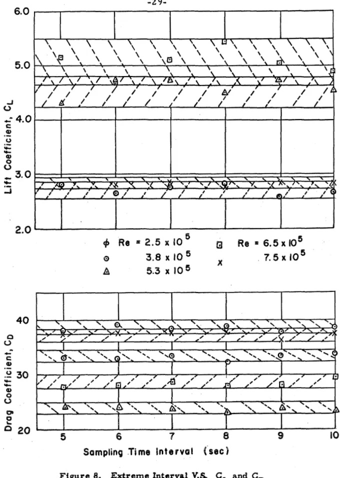
There a r e two questions l e f t to be answered. One i s whether the extreme value distribution is strongly influenced by the time in- t e r v a l of data collection. The other i s whether the initial distribu- tion is exponential. To examine the f i r s t question, the resultant f o r c e s in

e

= 90° (lift) and 0 = 180° (drag) f o r a period of 500 seconds were analyzed. The l i f t and drag coefficient a r e plotted v e r s u s dif- f e r e n t sampling time intervals in Fig. 8. The different sampling time interval s e e m s to have no effect on the e x t r e m e values. There- f o r e , the e x t r e m e value can be picked up by any convenient interval as long a s the flow condition r e m a i n s unchanged.

'9. DISCUSSION

Since Gumbel's extreme-value theory is based on the initial distribution being of a n exponential type, i t is n e c e s s a r y to examine the initial distribution by a n extensive data collection and analysis.

However, i f we a s s u m e that 87,500 observations did r e p r e s e n t a l a r g e sample, then the initial distribution can be obtained by usual means. A computer program was made to do this. The data used was absolute value of the lift coefficient (corresponding to the r e s u l - tant f o r c e in the direction perpendicular to the f r e e s t r e a m ) . The analysis shows that this distribution h a s a mean value of 69.629 and

;a standard deviation of r = 0.48484. The frequency function i s plotted i n Fig. 9. The experimental data m a y be compared with the normal distribution with the same mean and standard deviation a s shown in the figure. However, one m u s t r e a l i z e that since the variate lCL

1

i s positive, i t s distribution cannot be n o r m a l even if CL itself is normally distributed. The comparison therefore is incomplete, but i s offered f o r future examinations.

The experimental data used in this r e p o r t w e r e only from one section of the cylinder where the instrumentation was placed.

It is obvious that f o r a cantilever cylinder of finite length the fluc- tuating air loads will v a r y from one end to another. Refs. 9, 10, and 11 8 deal with this three-dimensional effect extensively, but

inconclusively. No detailea study sf the e x t r e m e p r e s s u r e variation along a three -dimensional body h a s been made. Evidently much r e m a i n s to be done in this field.

-1 5-

8. CONCLUSION

Gumbel's extreme value theory h a s been applied to many problems such a s the effective gust velocity and the extreme wind- speed (Ref. 8) and was proved adequate. This r e p o r t shows that the same theory is useful in the problem of predicting the fluctuating a i r load acting on a cylinder in a flow a t l a r g e Reynolds number.

The varied relationships between the e x t r e m e value envelope and the static and the root-mean- square curves a r e demonstrated in this r e p o r t . Ht i s shown that there a r e considerable differences between the static a i r load distribution and e x t r e m e air load distribution.

This information should be useful i n p r a c t i c a l design of cylindrical s t r u c t u r e s

.

F r o m F i g u r e s 2-6, i t i s s e e n that the e x t r e m e value envelope i s not entirely s i m i l a r to the root-mean-square curve f o r the p r e s

-

s u r e distribution around the circumference. Therefore the c u r r e n t practice of estimating the extreme value by multiplying the root- mean-square values with a uniform constant ( s a y 3 ~ ) cannot be a rigorously valid procedure. However, in all the c a s e s examined, the position around the circumference when the l a r g e s t extreme value of p r e s s u r e o c c u r s s e e m s to coincide with tihe point when the Barge st root -mean

-

square value o c c u r s

.

Fung, Y . C.

,

The Analysis of Wind-Induced Oscillations a t L a r g e and Tall Cylindrical S t r u c t u r e s " , Space Technology L a b o r a t o r i e s , Inc.

,

STL/TR -60-0000-09134, EM1 0-3 (June 1960).

Fung, Y . C.

,

l'Fluctuating Lift and Drag Acting on a Cylinder in a Flow a t Supercritical Reynolds Numbers"

,

Journal of

Aerospace Sciences, Vol. 27, No. 1 1 , pp. 801 -814. (November 1960).

Schmidt, L . V .

,

"Measurement of Fluctuating A i r Eoads on a C i r c u l a r Cylinder", Ph. D. T h e s i s , California Institute of Technology (1 963).

S p i t z e r , hi. E.

,

"Measurements of Unsteady P r e s s u r e and Wake Fluctuations f o r Flow over a Cylinder a t Supercritical Reynolds Numbers ! , A. E , T h e s i s , California Institute of Technology (1 965).

C r a m e r

,

H

. ,

Mathematical Methods s f S t a t i s t i c s q

' ,

Princeton University P r e s s , 1946, pp. 3'80-378.

Gumbel, E. J., "Statistics of E x t r e m e s " , Columbia University P r e s s , New York, 1958.

Chen, J. C.

,

"Study of Theory of E x t r e m e Values and an Application of Air Load to C y l i n d e r s s , preliminary r e p o r t s f Aeroelasticity and S t r u c t u r a l Dynamics. California Institute of TechnoPogy, September

P

965.

G m b e l , E. J .

,

and C a r l s o n , P. G.

,

"Extreme Values in Aeronautics", J o u r n a l of Aeronautical Sciences, VoP. 21, No.

6, pp. 389, June 1954.

Blackiston, H , S.

,

Tip Effects on Fluctuating A i r Eoads on a C i r c u l a r Cylinderf I , AIAA Fifth Annual S t r u c t u r e s and Materials Conference, pp. 146, A p r i l 1964.

Rainey

,

G . A.

,

s P r o g r e s s on the Launch-Vehicle Buffeting Problem", A M Fifth Annual S t r u c t u r e s and M a t e r i a l s Confer- ence, pp. 1 4 3 , A p r i l 1964.

BuelP, D. A.

,

"Some Sources of Ground-Wind Eoads in Launch Vehicle s t

,

AEAA Fifth Annual S t r u c t u r e s and Materials Confer

-

ence, pp, 1 7 8 , A p r i l 1964.

PROBABILITIES OF EXTREMES Worksheet 1

Plotting Position

- X

Nt1

Extr eme Cumulative

Frequency Extremes Square

X X 2

Worksheet 1 (continued)

Cumulative E x t r erne Plotting

F r e q u e n c y E x t r e m e s S q u a r e P o s i t i o n

Sum:

N = -

35' ^CXi

=

^74.3826

ZX: =

^159.3353

PROBABILITIES O F EXTREMES Worksheet 2

I. Mean and Standard Deviation:

~ e a n

'Ti=

2.125 Standard Deviation Sx= 0. 18946 I I. P a r a m e t e r s :

v

111 Line of Expected E x t r e m e s :

T

1. 0006 P. 582 PO. 2 0 . 589 100. 148. 811

F o r l a r g e s t value

\, N=

1.141 P

=

0. 19156

FOP next to l a r g e s t value A x , N - 1 -

-

^.759

($1 =

^0.12'743

P a r a m e t e r s f o r P r e s s u r e Coefficient

R e = 2. 5x10 3 . 8 ~ 1 0 5. 3x10 6. 5x10 7 . 5 ~ 1 0 5 8 q 5 p s f 10 p s f 20 p s f 30 psf 40 psf 0" - 0 , 9131 -6. 1213 -3. 1293 -0. 2405 t 3 . 11 58

l / a

-0. 3944 -0. 0626 ;O. 0246 -0. 01978

t o .

¹²⁴²

-1. 1814 -9. 4193 -8. 2690 - 6 . 0 9 4 3 -3. 0790 l o o 17, - 0 . 9 5 9 9 - 0 . 3 6 6 3 -0. 0439 -0. 0995 0, 1065 '

u t 3 . 9001 - 4 . 4404 -7. 1309 - 5 . 0 0 6 0 -2. 3902

l / a t o .

9976 -0. 3616 -0. 0756 -0. 1056 -0. 0466

30° -1, 9215 -5.2340 -3. 5880 -2. 3738 -0. 8098

n/a

-0.4151 -0. 1507 -0. 1269 -0. 0912 -0. 2065 -1. 7117 - 4 . 0 0 3 4 -3. 0587 - 2 . 6 5 4 5 ^{$ ,} -1. 4811 400 lya -0. 5060 -0. 1777 -0. 0745 -0.0917 -0. 0348 u + l . 3555 - 3 . 4 9 3 4 -5. 2368 - 5 . 0 6 0 9 -3. 5406 580

l / a t o .

^{2862 -0. 3566 -0. 1072 -0. 0216 -0. 1558}

u t 3 . 2109 -3. 5628 -5. 3074 - 5 . 8 6 5 7 -5. 2192 1 / a

t o .

^{3347 -0. 3738} -0. 1416 -0. 0479 -0. 1312

a o ~

u +4. 3306 - 3 . 9 3 4 5 -6. 8682 -7. 0183 -6. 2664

] / a

-to. 5898 -0. 6569 -0. 1 4 8 5 -0. 0801 -0. 1300 -6. 8368 - 5 . 9 6 9 4 - 5 . 9 3 6 1 - 5 . 2 1 6 5 $ 0 . 4 3 2 7 800 1 y a -0. 5690 -0. 1958 -0. 1105 -0. 1469

t o .

¹⁹⁹⁹

u t 4 . 2 2 1 4 -6. 1723 - 7 . 8 7 8 1 -7. 7787 -6. 6232

900

l / a t o .

³⁹⁰⁹ -0. 5378 -0. 1680 -0. 1174 -0. 1456

108" t 5 . 2 7 8 4 -4. 3065 -6. 7680 -7. 3900 -6. 1738 - 0 . 4 9 6 4

1

1 t o .

^{5 6 5 4 -0. 2066 -0. 2037 -0. 1864}

u - 3 . 4 5 2 1 -14.4222 - 9 . 9 7 8 9 -7. 9259 -4. 5334

"o"

^{1 / a -0. 9694 -0. 9837 -0. 7127} - 0 . 4 1 9 4 - 0 . 0 5 7 8 u $6, 3648 -7. 1 6 1 4 -8. 4080 -8. 3555 -5. 5783 n200 1 / a

t o .

1705 -0. 7087 -0. 2751 -0. 1565 - 0 . 0 0 1 1 u t 6 . 2 3 7 4 -3.3111 -6. 2858 -7. 0644 -5.4340 1300

l / a t o .

⁵⁷⁰² - 0 . 4 3 7 5 -0. 2819 -0. 4607 -0. 0690

140° -4.4586 -4. 1552 -6. 0659 -5. 5716 -3. 3114

] / a

-0. 9040 -0. 3275 -0. 1981 -0. 1761 -0, 01 46

u t 3 . 8734 -2. 27 - 4 . 8 0 2 3 - 5 , 3 9 5 8 -3. 9431 '500 1 / a

t o .

⁴⁸⁶⁰ -0.46;; -0. 0972 -0. 2086 -0. 0082 u t 4 . 1 6 6 3 - 1 . 7 3 9 4 -3. B 1 3 7 -3. 9476 - 3 , 0792 1 / a

t o .

^{5650 -0. 2504 -0. 1185 -0. 1746 -0. 1548}

u 4-4.336 t 3 . 213'7 -3. 1710 -4.1549 -3.1775

""

i/g, +0.435: 4-0. 1645 -0.1753 -0.1583 -0. 1264

-21

-

TABLE 2

P a r a m e t e r s for P r e s s u r e Coefficient

8 '4 5 psf 10 psf 20 psf 30 psf 40 psf

- 0 u 1.8101 3.4304 2. 3315 2.0345

Circurnferentiol Position, 0

(

degrees)

Figure 2. Extreme Envelope of C R e = 2 , 5 x 1 0 5

P.

Figure 3, Extreme Envelope of C

P .

R e = 3 , 8 x 1 0 5

.

68

90 928

IS0

rl) degrees

Figure 4, Extreme Envelope of

C

R e - 5 . 3 ~ 1 0 5 P

2 .o

0

-2.0 u

m

C1 C e

0 )

.-

(9

+

-40

Q

8

L

3

V) Vs <u

-6.0

&

-8.0

W M S

Value

Q S t a t i c Pressure

-88.0

0

60 90 120

180

Ci~cromfetenPiell Pssi

tion

,

⁶⁾

(degrees B

Figure 5. Extreme Envelope of @ R e ~ 6 . 5 x P O 5

P

Figure 6, Extreme Envelope of C

Re

+ 7,5x10 5

P

Sampling

.Ti me In

t

e

rvel

(set 1

Figure 8. Extreme Interval V.S

CL

and

CD