3 Binary Search Trees
Lioconcha castrensis shell, 2005. Michael T. Goodrich. Used with permission.
Contents
3.1 Searches and Updates . . . 91
3.2 Range Queries . . . 101
3.3 Index-Based Searching . . . 104
3.4 Randomly Constructed Search Trees . . . 107
3.5 Exercises . . . 110
Figure 3.1: A three-dimensional virtual environment. U.S. Army photo.
In three-dimensional video games and virtual environments, it is important to be able to locate objects relative to the other objects in their environment. For example, if the system is modeling a player driving a simulated vehicle through a virtual war zone, it is useful to know where that vehicle is relative to various obstacles and other players. Such nearby objects are useful for the sake of rendering a scene or identifying targets, for example. (See Figure 3.1.)
Of course, one way to do such a reference check for some object,x, relative to a virtual environment is to comparexto every other object in the environment. For an environment made up ofn objects, such a search would requireO(n)object- object comparisons forx; hence, doing such a search for every object, x, would take O(n2) time, which is expensive. Such a computation for a given objectx is not taking advantage of the fact that it is likely that there are potentially large groups of objects far fromx. It would be nice to quickly dismiss such groups as being of low interest, rather than comparing each one toxindividually.
For such reasons, many three-dimensional video games and virtual environ- ments, including the earliest versions of the gameDoom, create a partitioning of space using a binary tree, by applying a technique known asbinary space parti- tioning. To create such a partitioning, we identify a plane,P, that divides the set of objects into two groups of roughly equal size—those objects to the left ofP and those objects to the right ofP. Then, for each group, we recursively subdivide them with other separating planes until the number of objects in each subgroup is small enough to handle as individuals. Given such a binary space partition (or BSP) tree, we can then locate any object in the environment simply by locating it relative to P, and then recursively locating it with respect to the objects that fall on the same side ofP as it does. Such BSP tree partitions represent a three-dimensional envi- ronment using the data structure we discuss in this chapter, thebinary search tree, in that a BSP tree is a binary tree that stores objects at its nodes in a way that allows us to perform searches by making left-or-right decisions at each of its nodes.
3.1 Searches and Updates
Suppose we are given an ordered set,S, of objects, represented as key-value pairs, for which we would like to locate query objects, x, relative to the objects in this set. That is, we would like to identify the nearest neighbors ofxinS, namely, the smallest object greater thanx in S and the largest object smaller than x inS, if these objects exist. One of the simplest ways of storingS in this way is to store the elements ofSin order in an arrayA. Such a representation would allow us, for example, to identify theith smallest key, simply by looking up the key of the item stored in cellA[i]. In other words, if we needed a method,key(i), for accessing the key of theith smallest key-value pair, orelem(i), the element that is associated with this key, then we could implement these methods in constant time given the representation of S in sorted order in the array A. In addition, if we store the elements ofSin such a sorted array,A, then we know that the item at indexihas a key no smaller than keys of the items at indices less thaniand no larger than keys of the items at indices larger thani.
The Binary Search Algorithm
This observation allows us to quickly “home in” on a search keykusing a variant of the children’s game “high-low.” We call an itemIofSacandidateif, at the current stage of the search, we cannot rule out thatI has key equal tok. The algorithm that results from this strategy is known asbinary search.
There are several ways to implement this strategy. The method we describe here maintains two parameters, low and high, such that all the candidate items have index at leastlowand at mosthighinS. Initially,low= 1andhigh=n, and we letkey(i)denote the key at indexi, which haselem(i)as its element. We then comparekto the key of the median candidate, that is, the item with index
mid=⌊(low+high)/2⌋.
We consider three cases:
• Ifk=key(mid), then we have found the item we were looking for, and the search terminates successfully returningelem(mid).
• Ifk <key(mid), then we recur on the first half of the vector, that is, on the range of indices fromlowtomid−1.
• Ifk >key(mid), we recursively search the range of indices frommid+ 1to high.
This binary search method is given in detail in Algorithm 3.2. To initiate a search for key k on an n-item sorted array, A, indexed from 1 to n, we call BinarySearch(A, k,1, n).
AlgorithmBinarySearch(A, k,low,high):
Input: An ordered array, A, storing n items, whose keys are accessed with method key(i) and whose elements are accessed with method elem(i); a search keyk; and integerslowandhigh
Output: An element ofAwith keykand index betweenlowandhigh, if such an element exists, and otherwise the special elementnull
iflow>highthen returnnull else
mid← ⌊(low+high)/2⌋
if k=key(mid) then returnelem(mid) else if k <key(mid) then
returnBinarySearch(A, k,low,mid−1) else
returnBinarySearch(A, k,mid+ 1,high)
Algorithm 3.2:Binary search in an ordered array.
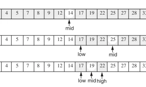
We illustrate the binary search algorithm in Figure 3.3.
2 4 5 7 8 9 12 14 17 19 22 25 27 28 33 37
2 4 5 7 8 9 12 14 17 19 22 25 27 28 33 37
2 4 5 7 8 9 12 14 17 19 22 25 27 28 33 37
2 4 5 7 8 9 12 14 17 19 22 25 27 28 33 37
low mid high
mid high low
low midhigh
low=mid=high
Figure 3.3: Example of a binary search to search for an element with key22 in a sorted array. For simplicity, we show the keys but not the elements.
Analyzing the Binary Search Algorithm
Considering the running time of binary search, we observe that a constant number of operations are executed at each recursive call. Hence, the running time is pro- portional to the number of recursive calls performed. A crucial fact is that, with each recursive call, the number of candidate items still to be searched in the array Ais given by the valuehigh−low+ 1. Moreover, the number of remaining candi- dates is reduced by at least one half with each recursive call. Specifically, from the definition ofmid, the number of remaining candidates is either
(mid−1)−low+ 1 =
low+high 2
−low≤ high−low+ 1 2 or
high−(mid+ 1) + 1 =high−
low+high 2
≤ high−low+ 1
2 .
Initially, the number of candidate isn; after the first call toBinarySearch, it is at mostn/2; after the second call, it is at mostn/4; and so on. That is, if we let a function,T(n), represent the running time of this method, then we can characterize the running time of the recursive binary search algorithm as follows:
T(n)≤
b ifn <2 T(n/2) +b else,
wherebis a constant. In general, this recurrence equation shows that the number of candidate items remaining after each recursive call is at mostn/2i. (We discuss recurrence equations like this one in more detail in Section 11.1.) In the worst case (unsuccessful search), the recursive calls stop when there are no more candidate items. Hence, the maximum number of recursive calls performed is the smallest integermsuch thatn/2m<1. In other words (recalling that we omit a logarithm’s base when it is2),m >logn. Thus, we havem=⌊logn⌋+ 1, which implies that BinarySearch(A, k,1, n)runs inO(logn)time.
The space requirement of this solution is Θ(n), which is optimal, since we have to store thenobjects somewhere. This solution is only efficient if the setSis static, however, that is, we don’t want to insert or delete any key-value pairs inS.
In the dynamic case, where we want to perform insertions and deletions, then such updates takeO(n)time. The reason for this poor performance in an insertion, for instance, is due to our need to move elements inAgreater than the insertion key in order to keep all the elements inAin sorted order, similar to the methods described in Section 2.2.1. Thus, using an ordered array to store elements to support fast searching only makes sense for the sake of efficiency if we don’t need to perform insertions or deletions.
3.1.1 Binary Search Tree Definition
The data structure we discuss in this section, the binary search tree, applies the motivation of the binary search procedure to a tree-based data structure, to support update operations more efficiently. We define a binary search tree to be a binary tree in which each internal nodevstores an elementesuch that the elements stored in the left subtree ofvare less than or equal to e, and the elements stored in the right subtree ofv are greater than or equal toe. Furthermore, let us assume that external nodes store no elements; hence, they could in fact benullor references to a specialNULL NODEobject.
An inorder traversal of a binary search tree visits the elements stored in such a tree in nondecreasing order. A binary search tree supports searching, where the question asked at each internal node is whether the element at that node is less than, equal to, or larger than the element being searched for.
We can use a binary search treeT to locate an element with a certain valuex by traversing down the treeT. At each internal node we compare the value of the current node to our search elementx. If the answer to the question is “smaller,”
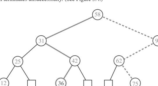
then the search continues in the left subtree. If the answer is “equal,” then the search terminates successfully. If the answer is “greater,” then the search continues in the right subtree. Finally, if we reach an external node (which is empty), then the search terminates unsuccessfully. (See Figure 3.4.)
12 36 75
25 42 62
31 90
58
Figure 3.4: A binary search tree storing integers. The thick solid path drawn with thick lines is traversed when searching (successfully) for36. The thick dashed path is traversed when searching (unsuccessfully) for70.
3.1.2 Searching in a Binary Search Tree
Formally, abinary search treeis a binary tree,T, in which each internal nodevof T stores a key-value pair,(k, e), such that keys stored at nodes in the left subtree ofvare less than or equal tok, while keys stored at nodes in the right subtree ofv are greater than or equal tok.
In Algorithm 3.5, we give a recursive methodTreeSearch, based on the above strategy for searching in a binary search treeT. Given a search keykand a node vofT, methodTreeSearchreturns a node (position)wof the subtreeT(v)ofT rooted atv, such that one of the following two cases occurs:
• wis an internal node ofT(v)that stores keyk.
• wis an external node ofT(v). All the internal nodes ofT(v)that precedew in the inorder traversal have keys smaller thank, and all the internal nodes of T(v)that followwin the inorder traversal have keys greater thank.
Thus, a methodfind(k), which returns the element associated with the keyk, can be performed on a set of key-value pairs stored in a binary search tree,T, by calling the method TreeSearch(k, T.root()) onT. Letw be the node ofT returned by this call of theTreeSearchmethod. If nodewis internal, we return the element stored atw; otherwise, ifwis external, then we returnnull.
AlgorithmTreeSearch(k, v):
Input:A search keyk, and a nodevof a binary search treeT
Output:A nodewof the subtreeT(v)ofTrooted atv, such that eitherwis an internal node storing keykorwis the external node where an item with key kwould belong if it existed
ifvis an external nodethen returnv
if k=key(v) then returnv
else if k <key(v) then
returnTreeSearch(k, T.leftChild(v)) else
returnTreeSearch(k, T.rightChild(v))
Algorithm 3.5:Recursive search in a binary search tree.
The analysis of the running time of this algorithm is simple. The binary tree search algorithm executes a constant number of primitive operations for each node it traverses in the tree. Each new step in the traversal is made on a child of the previous node. That is, the binary tree search algorithm is performed on the nodes of a path ofT that starts from the root and goes down one level at a time. Thus, the
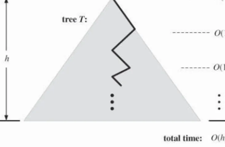
number of such nodes is bounded byh+ 1, where his the height ofT. In other words, since we spendO(1)time per node encountered, the search method runs in O(h)time, wherehis the height of the binary search treeT. (See Figure 3.6.)
Figure 3.6: Illustrating the running time of searching in a binary search tree. The figure uses standard visualization shortcuts of viewing a binary search tree as a big triangle and a path from the root as a zig-zag line.
Admittedly, the heighthofT can be as large asn, but we expect that it is usu- ally much smaller. The best we can do for the height,h, is⌈log(n+ 1)⌉(see Exer- cise C-3.5), and we would hope that in most caseshwould in fact beO(logn). For instance, we show below, in Section 3.4, that a randomly constructed binary search tree will have heightO(logn)with high probability. For now, though, consider a binary search tree,T, storingnitems, such that, for each nodevinT, each ofv’s children store at most three-quarters as many items in their subtrees asvdoes. Lots of binary search trees could have this property, and, for any such tree, its height, H(n), would satisfy the following recurrence equation:
H(n)≤
1 ifn <2 H(3n/4) + 1 else.
In other words, a child of the root stores at most(3/4)nitems in its subtree, any of its children store at most(3/4)2nitems in their subtrees, any of their children store at most(3/4)3nitems in their subtrees, and so on. Thus, since multiplying by3/4is the same as dividing by4/3, this implies thatH(n)is at most⌈log4/3n⌉, which is O(logn). Intuitively, the reason we achieve a logarithmic height forT in this case is that the subtrees rooted at each child of a node inT have roughly
“balanced” sizes.
We show in the next chapter how to maintain an upper bound ofO(logn)on the height of a search treeT, by maintaining similar notions of balance, even while performing insertions and deletions. Before we describe such schemes, however, let us describe how to do insertions and deletions in a standard binary search tree.
3.1.3 Insertion in a Binary Search Tree
Binary search trees allow implementations of theinsert andremove operations using algorithms that are fairly straightforward, but not trivial. To perform the operationinsert(k, e)in a binary search treeT, to insert a key-value pair, (k, e), we perform the following algorithm (which works even if the tree holds multiple key-value pairs with the same key):
Letw←TreeSearch(k, T.root()) whilewis an internal nodedo
// There is item with key equal tokinT in this case Letw←TreeSearch(k, T.leftChild(w))
Expandwinto an internal node with two external-node children Store(k, e)atw
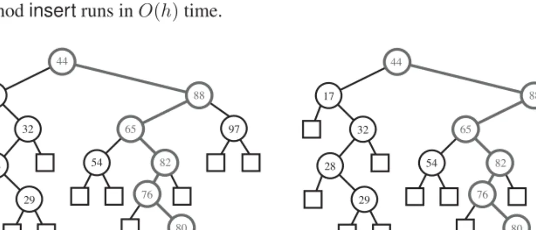
The above insertion algorithm eventually traces a path from the root ofT down to an external node,w, which is the appropriate place to insert an item with keyk based on the ordering of the items stored inT. This node then gets replaced with a new internal node accommodating the new item. Hence, an insertion adds the new item at the “bottom” of the search treeT. An example of insertion into a binary search tree is shown in Figure 3.7.
The analysis of the insertion algorithm is analogous to that for searching. The number of nodes visited is proportional to the heighthofTin the worst case, since we spendO(1)time at each node visited. Thus, the above implementation of the methodinsertruns inO(h)time.
97 44
17 88
32 65
54 82
28
29 76
80
(a) (b)
97 44
17 88
32 65
54 82
28
29 76
80 78
Figure 3.7: Insertion of an item with key78into a binary search tree. Finding the position to insert is shown in (a), and the resulting tree is shown in (b).
3.1.4 Deletion in a Binary Search Tree
Performing a remove(k) operation, to remove an item with key k from a binary search treeT is a bit more complex than the insertion algorithm, since we do not wish to create any “holes” in the treeT. Such a hole, where an internal node would not store an element, would make it difficult if not impossible for us to correctly perform searches in the binary search tree. Indeed, if we have many removals that do not restructure the treeT, then there could be a large section of internal nodes that store no elements, which would confuse any future searches. Thus, we must implement item deletion to avoid this situation.
The removal operation starts out simple enough, since we begin by execut- ing algorithm TreeSearch(k, T.root()) on T to find a node storing key k. If TreeSearchreturns an external node, then there is no element with keyk inT, and we return the special elementnull and are done. If TreeSearchreturns an internal nodewinstead, thenwstores an item we wish to remove.
We distinguish two cases (of increasing difficulty) of how to proceed based on whetherwis a node that is easily removed:
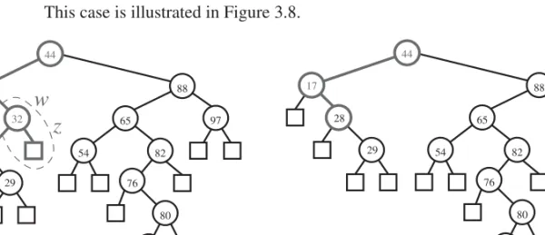
• If one of the children of nodewis an external node, say nodez, we simply removewandz from T, and replace w with the sibling ofz (which is an operation calledremoveAboveExternal(z)in Section 2.3.4).
This case is illustrated in Figure 3.8.
97 44
17 88
32 65
54 82
28
29 76
80
78
(a) (b)
w
z
9744
17 88
65
54 82
28 29
76 80 78
Figure 3.8: Deletion from the binary search tree of Figure 3.7b, where the key to remove (32) is stored at a node (w) with an external child: (a) shows the tree before the removal, together with the nodes affected by the operation that removes the external node,z, and its parent,w, replacingwwith the sibling ofz; (b) shows the treeT after the removal.
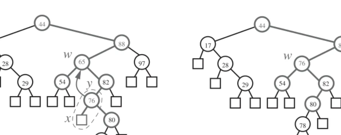
• If both children of nodeware internal nodes, we cannot simply remove the nodewfromT, since this would create a “hole” inT. Instead, we proceed as follows (see Figure 3.9):
1. We find the first internal nodey that followswin an inorder traversal ofT. Node y is the left-most internal node in the right subtree ofw, and is found by going first to the right child ofwand then downTfrom there, following left children. Also, the left childxofyis the external node that immediately follows nodewin the inorder traversal ofT. 2. We save the element stored at win a temporary variable t, and move
the item ofyintow. This action has the effect of removing the former item stored atw.
3. We remove x and y from T by replacing y with x’s sibling, and removing both x and y from T (which is equivalent to opera- tion removeAboveExternal(x) onT, using the terminology of Sec- tion 2.3.4).
4. We return the element previously stored at w, which we had saved in the temporary variablet.
97 44
17 88
76
54 82
28
29
80
78
(a) (b)
97
w
44
17 88
65
54 82
28
29
76 80
78
w y x
Figure 3.9: Deletion from the binary search tree of Figure 3.7b, where the key to remove (65) is stored at a node whose children are both internal: (a) before the removal; (b) after the removal.
Note that in Step 1 above, we could have selectedy as the right-most internal node in the left subtree ofw.
The analysis of the removal algorithm is analogous to that of the insertion and search algorithms. We spendO(1)time at each node visited, and, in the worst case, the number of nodes visited is proportional to the heighthofT. Thus, in a binary search tree,T, theremovemethod runs inO(h)time, wherehis the height ofT.
3.1.5 The Performance of Binary Search Trees
A binary search treeT is an efficient implementation of an ordered set ofnkey- value pairs but only if the height ofTis small. For instance, ifT is balanced so that it has height O(logn), then we get logarithmic-time performance for the search and update operations described above. In the worst case, however,T could have height as large asn; hence, it would perform like an ordered linked list in this case.
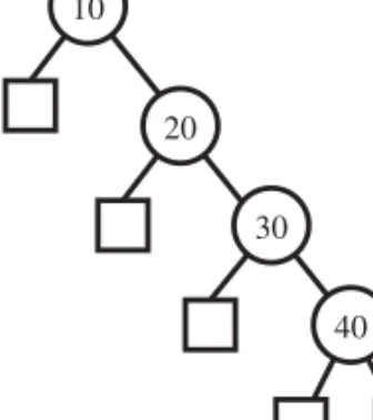
Such a worst-case configuration arises, for example, if we insert a set of keys in increasing order. (See Figure 3.10.)
10
20
30
40
Figure 3.10:Example of a binary search tree with linear height, obtained by insert- ing keys in increasing order.
To sum up, we characterize the performance of the binary search tree data struc- ture in the following theorem.
Theorem 3.1: A binary search treeT with heighthfornkey-element items uses O(n) space and executes the operations find, insert, and removeeach in O(h) time.
Ideally, of course, we would like our binary search tree to have heightO(logn), and there are several ways to achieve this goal, including several that we explore in the next chapter. For instance, as we explore in this chapter (in Section 3.4), if we construct a binary search tree,T, by inserting a set ofnitems in random order, then the height ofT will be O(logn)with high probability. Alternatively, if we have our entire set,S, ofnitems available, then we can sortSand build a binary search tree, T, with heightO(logn) from the sorted listing of S (see Exercise A-3.2).
In addition, if we already have a binary search tree, T, of O(logn) height, and thereafter only perform deletions fromT, then each of those deletion operations will run inO(logn)time (although interspersing insertions and deletions can lead to poor performance if we don’t have some way to maintain balance). There are a number of other interesting operations that can be done using binary search trees, however, besides simple searches and insertions and deletions.
3.2 Range Queries
Besides the operations mentioned above, there are other interesting operations that can be performed using a binary search tree. One such operation is the range queryoperation, where, we are given an ordered set,S, of key-value pairs, stored in a binary search tree,T, and are asked to perform the following query:
findAllInRange(k1, k2): Return all the elements stored inT with keyksuch that k1≤k≤k2.
Such an operation would be useful, for example, to find all cars within a given price range in a set of cars for sale. Suppose, then, that we have a binary search treeTrepresentingS. To perform thefindAllInRange(k1, k2)operation, we use a recursive method,RangeQuery, that takes as arguments,k1 andk2, and a nodev inT. If nodevis external, we are done. If nodevis internal, we have three cases, depending on the value ofkey(v), the key of the item stored at nodev:
• key(v)< k1: We recursively search the right child ofv.
• k1 ≤ key(v) ≤ k2: We reportelement(v)and recursively search both chil- dren ofv.
• key(v)> k2: We recursively search the left child ofv.
We describe the details of this search procedure in Algorithm 3.11 and we illus- trate it in Figure 3.12. We perform operationfindAllInRange(k1, k2)by calling RangeQuery(k1, k2, T.root()).
AlgorithmRangeQuery(k1, k2, v):
Input:Search keysk1andk2, and a nodevof a binary search treeT
Output: The elements stored in the subtree ofT rooted atvwhose keys are in the range[k1, k2]
ifT.isExternal(v)then return∅
if k1 ≤key(v)≤k2 then
L←RangeQuery(k1, k2, T.leftChild(v)) R←RangeQuery(k1, k2, T.rightChild(v)) returnL∪ {element(v)} ∪R
else if key(v)< k1 then
returnRangeQuery(k1, k2, T.rightChild(v)) else if k2 <key(v) then
returnRangeQuery(k1, k2, T.leftChild(v))
Algorithm 3.11: The method for performing a range query in a binary search tree.
12
18 55 81
99 68
23 42 74 90
21
37
49
61
30 80
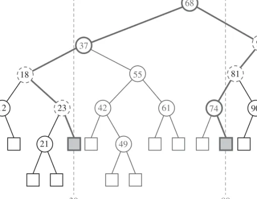
Figure 3.12:A range query using a binary search tree for the keysk1 = 30andk2 = 80. PathsP1andP2 of boundary nodes are drawn with thick lines. The boundary nodes storing items with key outside the interval [k1, k2]are drawn with dashed lines. There are four internal inside nodes.
Intuitively, the methodRangeQueryis a modification of the standard binary- tree search method (Algorithm 3.5) to search for the keys betweenk1andk2, inclu- sive. For the sake of simplifying our analysis, however, let us assume thatT does not contain items with keyk1ork2.
Let P1 be the search path traversed when performing a search in tree T for keyk1. PathP1starts at the root ofT and ends at an external node ofT. Define a pathP2similarly with respect tok2. We identify each nodevofT as belonging to one of following three groups (see Figure 3.12):
• Nodevis aboundary nodeifvbelongs toP1 orP2; a boundary node stores an item whose key may be inside or outside the interval[k1, k2].
• Node v is an inside node if v is not a boundary node and v belongs to a subtree rooted at a right child of a node ofP1or at a left child of a node ofP2; an internal inside node stores an item whose key is inside the interval[k1, k2].
• Nodevis anoutside nodeifvis not a boundary node andvbelongs to a sub- tree rooted at a left child of a node ofP1or at a right child of a node ofP2; an internal outside node stores an item whose key is outside the interval[k1, k2].
Analysis of the Range Query Operation
Consider an execution of the algorithmRangeQuery(k1, k2, r), whereris the root ofT. We traverse a path of boundary nodes, calling the algorithm recursively either on the left or on the right child, until we reach either an external node or an internal nodew(which may be the root) with key in the range[k1, k2]. In the first case (we reach an external node), the algorithm terminates returning the empty set. In the second case, the execution continues by calling the algorithm recursively at both ofw’s children. We know that nodewis the bottommost node common to paths P1 andP2. For each boundary nodevvisited from this point on, we either make a single call at a child ofv, which is also a boundary node, or we make a call at one child ofvthat is a boundary node and the other child that is an inside node. Once we visit an inside node, we will visit all of its (inside node) descendants.
Since we spend a constant amount of work per node visited by the algorithm, the running time of the algorithm is proportional to the number of nodes visited.
We count the nodes visited as follows:
• We visit no outside nodes.
• We visit at most2h+ 1boundary nodes, whereh is the height ofT, since boundary nodes are on the search pathsP1andP2and they share at least one node (the root ofT).
• Each time we visit an inside nodev, we also visit the entire subtree Tv of T rooted at v and we add all the elements stored at internal nodes of Tv to the reported set. If Tv holds sv items, then it has2sv + 1 nodes. The inside nodes can be partitioned intoj disjoint subtreesT1, . . . , Tj rooted at children of boundary nodes, wherej ≤2h. Denoting withsi the number of items stored in treeTi, we have that the total number of inside nodes visited is equal to
j
i=1
(2si+ 1) = 2s+j≤2s+ 2h.
Therefore, at most 2s + 4h + 1 nodes of T are visited and the operation findAllInRangeruns inO(h+s)time. We summarize:
Theorem 3.2: A binary search tree of height h storing n items supports range query operations with the following performance:
• The space used isO(n).
• Operation findAllInRangetakes O(h+s) time, wheresis the number of elements reported.
• Operationsinsertandremoveeach takeO(h)time.
3.3 Index-Based Searching
We began this chapter by discussing how to search in a sorted array, A, which allows us to quickly identify theith smallest item in the array simply by indexing the cellA[i]. As we mentioned, a weakness of this array representation is that it doesn’t support efficient updates, whereas a binary search tree allows for efficient insertions and deletions. But when we switched to a binary search tree, we lost the ability to quickly find theith smallest item in our set. In this section, we show how to regain that ability with a binary search tree.
Suppose, then, that we wish to support the following operation on a binary search tree,T, storingnkey-value pairs:
select(i): Return the item withith smallest key, for1≤i≤n.
For example, ifi= 1, then we would return the minimum item, ifi=n, then we would return the maximum, and ifi = ⌈n/2⌉, then we would return the median (assumingnis odd).
The main idea for a simple way to support this method is to augment each node,v, inT so as to add a new field,nv, to that node, where
• nv is the number of items stored in the subtree ofT rooted atv.
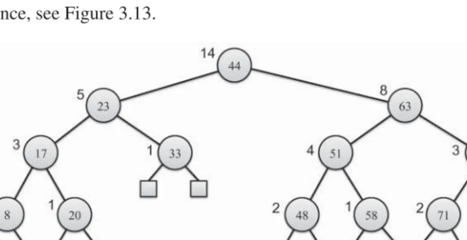
For instance, see Figure 3.13.
Figure 3.13: A binary search tree augmented so that each node, v, stores a count, nv, of the number of items stored in the subtree rooted atv. We show the key for each node inside that node and thenv value of each node next to the node, except for external nodes, which each have annvcount of0.
Searching and Updating Augmented Binary Search Trees
Having defined thenv count for each node in a binary search tree,T, we need to maintain it during updates toT. Fortunately, such updates are easy.
First, note that thenv count for any external node is0, so we don’t even need to store an actualnv field for external nodes (especially if they arenull objects).
To keep thenv counts for internal nodes up to date, we simply need to modify the insertion and deletion methods as follows:
• If we are doing an insertion at a node, w, in T (which was previously an external node), then we setnw = 1and we increment thenv count for each nodevthat is an ancestor ofw, that is, on the path fromwto the root ofT.
• If we are doing a deletion at a node,w, inT, then we decrement thenv count for each nodevthat is on the path fromw’s parent to the root ofT.
In either the insertion or deletion case, the additional work needed to perform the updates tonv counts takesO(h)time, where his the height ofT. This updating takes an additional amount of time that isO(h), wherehis the height ofT, because we spend an additional amount ofO(1)time for each node fromwto the root ofT in either case. (See Figure 3.14.)
Figure 3.14: A update in an a binary search tree augmented so that each node,v, stores a count,nv, of the number of items stored in the subtree rooted atv. We show the path taken, along withnv updates, during this update, which is an insertion of a node with key27in the tree from Figure 3.13.
Let us consider how to perform methodselect(i) on a tree,T, augmented as described above. The main idea is to search down the tree,T, while maintaining the value ofiso that we are looking for theith smallest key in the subtree we are still searching in. We do this by calling theTreeSelect(i, r, T), shown in Algo- rithm 3.15, wherer is the root ofT. Note that this algorithm assumes that thenv count for any external node is0. (See Figure 3.16.)
AlgorithmTreeSelect(i, v, T):
Input:Search indexiand a nodevof a binary search treeT
Output:The item withith smallest key stored in the subtree ofTrooted atv Letw←T.leftChild(v)
ifi≤nwthen
returnTreeSelect(i, w, T) else if i=nw+ 1 then
return(key(v),element(v)) else
returnTreeSelect(i−nw−1, T.rightChild(v), T) Algorithm 3.15: TheTreeSelectalgorithm.
The correctness of this algorithm follows from the fact that we are always main- tainingito be the index of theith smallest item in the subtree we are searching in, so that the item returned will be the correct index. In particular, note that when we recursively search in a right subtree, we first subtract the count of the number of items stored in the left subtree and the parent. The running time for performing this query isO(h), wherehis the height ofT, since we spendO(1)time per level ofT in our search to the node storing theith smallest key.
Figure 3.16: A search for the 10th smallest item in a binary search tree augmented so that each node,v, stores a count,nv, of the number of items stored in the subtree rooted atv. We show the path taken during this search, along with the value,i, that is maintained during this search.
3.4 Randomly Constructed Search Trees
Suppose we construct a binary search tree, T, by a sequence of insertions of n distinct, random keys. Since the only thing that impacts the structure ofT is the relative order of the keys, we can assume, without loss of generality, that the keys involved are the integers from1ton. That is, we can assume that we are given a random permutation,P, of the keys in the set{1,2, . . . , n}, where all permutations are equally likely, and are asked to build the binary search tree,T, by inserting the keys inP in the given order.
Letvjdenote the node inTthat holds the item with keyj, and letD(vj)denote the depth ofvj inT. Note thatD(vj)is a random variable, sinceT is constructed at random (based onP). DefineXi,j to be a 0-1 indicator random variable that is equal to 1 if and only ifviis an ancestor ofvj, where, for the sake of this analysis, we consider a node to be an ancestor of itself. That is,Xi,i= 1. We can write
D(vj) =
n
i=1
Xi,j − 1,
since the depth of a node is equal to the number of its proper ancestors. Thus, to de- rive a bound on the expected value ofD(vj), we need to determine the probability thatXi,j is1.
Lemma 3.3: The nodeviis an ancestor of the nodevjinT if and only ifiappears earliest inPof any integer inRi,j, the range of integers betweeniandj, inclusive.
Proof: Ifiappears earliest inP of any integer inRi,j, then, by definition, it is inserted intoT before any of these integers. Thus, at the time whenj is inserted intoT, and we performjinT, we must encounter the nodevias our depthD(vi) comparison, since there is no other element fromRi,j at a higher level inT.
Suppose, on the other hand, thatiappears earliest inP of any integer inRi,j. Theniis inserted into T before any item with a key in this range; hence, for the search forj, we will encountervi at some point along the way, sincej has to be located into this interval and, at the depth ofvi, there is no other element fromRi,j to use as a comparison key.
This fact allows us to then derive the probability that anyXi,j is1, as follows.
Lemma 3.4: LetXi,jbe defined as above. ThenPr(Xi,j = 1) = 1/(|i−j|+1).
Proof: There are |i−j|+ 1items in the range fromitoj, inclusive, and the probability thatiappears earliest inP of all of them is1over this number, since all the numbers in this range have an equal and independent probability of being earliest inP. The proof follows, then, from this fact and Lemma 3.3.
An Analysis Based on Harmonic Numbers
In addition to the above lemmas, our analysis of a randomly constructed binary search tree also involves harmonic numbers. For any integern≥1, we define the nthharmonic number,Hn, as
Hn=
n
i=1
1 i, for which it is well known thatHnisO(logn). In fact,
lnn≤Hn≤1 + lnn, as we explore in Exercise C-3.11.
Harmonic numbers are important in our analysis, because of the following.
Lemma 3.5:
E[D(vj)] ≤ Hj+Hn−j+1−1.
Proof: To see this relationship, note that, by the linearity of expectation, E[D(vj)] =
n
i=1
E[Xi,j] − 1
=
j
i=1
E[Xi,j] +
n
i=j+1
E[Xi,j] − 1
=
j
i=1
1 j−i+ 1 +
n
i=j+1
1
i−j+ 1 − 1
≤
j
k=1
1 k +
n−j+1
k=1
1 k − 1
= Hj+Hn−j+1−1.
So, in other words, the expected depth of any node in a randomly constructed binary search tree withnnodes isO(logn). Or, put another way, the average depth of the nodes in a randomly constructed binary search tree isO(logn).
Bounding the Overall Height with High Probability
In addition to the above bound for the average depth of a randomly constructed binary search tree, we might also be interested in bounding the overall height of such a tree,T, which is equal to the maximum depth of any node inT. In order to analyze this maximum depth of a node inT, let us utilize the following Chernoff bound (see Exercise C-19.14).
Let X1, X2, . . . , Xn be a set of mutually independent indicator random vari- ables, such that eachXi is1with some probabilitypi > 0 and0otherwise. Let X = n
i=1Xi be the sum of these random variables, and letµ′ denote an upper bound on the mean ofX, that is,E(X)≤µ′. Then, forδ >0,
Pr(X >(1 +δ)µ′)<
eδ
(1 +δ)(1+δ) µ′
. Using this bound, we can derive the following theorem.
Theorem 3.6: If T is a randomly constructed binary search tree with n > 4 nodes, then the height ofT isO(logn)with probability at least1−1/n.
Proof: Recall that D(vj) = n
i=1Xi,j − 1. LetLj = j−1
i=1Xi,j denote the “left” part of this sum and Rj = n
i=j+1Xi,j denote the “right” part, with both leaving off the termXj,j. Then D(vj) = Lj +Rj. So, by symmetry, it is sufficient for us to boundRj, since a similar bound will hold forLj. The important observation is that all of theXi,jterms in the definition ofRj are independent 0-1 random variables. This independence is due to the fact that whetheriis chosen first inP from{j, j+ 1, . . . , i}has no bearing on whether i+ 1 is chosen first inP from{j, j+ 1, . . . , i, i+ 1}. Moreover, E[Rj] = Hn−j+1 ≤ Hn. Thus, by the above Chernoff bound, forn >4,
Pr(Rj >4Hn) <
e3 44
Hn
≤ 1 n2.5,
sinceHn ≥ lnn. Therefore, Pr(D(vj) > 8Hn) ≤ 2/n2.5, which implies that the probability thatanynode inT has depth more than8Hnis at most2n/n2.5 = 2/n1.5. Sincen >4andHnisO(logn), this establishes the theorem.
So, if we construct a binary search tree,T, by inserting a set ofndistinct items in random order, then, with high probability, the height ofT will beO(logn).
The Problem with Deletions
Unfortunately, if we intersperse random insertions with random deletions, using the standard insertion and deletion algorithms given above, then the expected height of the resulting tree isΘ(n1/2), notO(logn). Indeed, it has been reported that a major database company experienced poor performance of one its products because of an issue with maintaining the height of a binary search tree to beO(logn)even while allowing for deletions. Thus, if we are hoping to achieveO(logn) depth for the nodes in a binary search tree that is subject to both insertions and deletions, even if these operations are for random keys, then we need to do more than simply performing the above standard insertion and deletion operations. For example, we could use one of the balanced search tree strategies discussed in the next chapter.
3.5 Exercises
Reinforcement
R-3.1 Suppose you are given the arrayA = [1,2,3,4,5,6,7,8,9,10,11,12], and you then perform the binary search algorithm given in this chapter to find the number 8. Which numbers in the arrayAare compared against the number8?
R-3.2 Insert items with the following keys (in the given order) into an initially empty binary search tree: 30, 40, 50, 24, 8, 58, 48, 26, 11, 13. Draw the tree that results.
R-3.3 Suppose you have a binary search tree,T, storing numbers in the range from 1 to 500, and you do a search for the integer 250. Which of the following sequences are possible sequences of numbers that were encountered in this search. For the ones that are possible, draw the search path, and, for the ones that are impossible, say why.
a. (2, 276, 264, 270, 250) b. (100, 285, 156, 203, 275, 250) c. (475, 360, 248, 249, 251, 250) d. (450, 262, 248, 249, 270, 250)
R-3.4 SupposeTis a binary search tree of height4(including the external nodes) that is storing all the integers in the range from 1 to 15, inclusive. Suppose further that you do a search for the number 11. Explain why it is impossible for the sequence of numbers you encounter in this search to be(9,12,10,11).
R-3.5 Draw the binary search trees of minimum and maximum heights that store all the integers in the range from1to7, inclusive.
R-3.6 Give a pseudocode description of an algorithm to find the element with smallest key in a binary search tree. What is the running time of your method?
R-3.7 Draw the binary search tree that results from deleting items with keys 17, 28, 54, and 65, in this order, from the tree shown in Figure 3.7b.
R-3.8 A certain Professor Amongus claims that the order in which a fixed set of ele- ments is inserted into a binary search tree does not matter—the same tree results every time. Give a small example that proves Professor Amongus wrong.
R-3.9 Suppose you are given a sorted set,S, ofnitems, stored in a binary search tree.
How many different range queries can be done where both of the values,k1and k2, in the query range[k1, k2]are members ofS?
R-3.10 Suppose that a binary search tree,T, is constructed by inserting the integers from 1tonin this order. Give a big-Oh characterization of the number of comparisons that were done to constructT.
R-3.11 Suppose you are given a binary search tree,T, which is constructed by inserting the integers in the set{1,2, . . . , n}in a random order intoT, where all permu- tations of this set are equally likely. What is the average running time of then performing aselect(i)operation onT?
R-3.12 If one has a set,S, ofnitems, wherenis even, then the median item inSis the average of theith and(i+ 1)st smallest elements inS, wherei=n/2. Describe an efficient algorithm for computing the median of such a setSthat is stored in a binary search tree,T, where each node,v, inTis augmented with a count,nv, which stores the number of items stored in the subtree ofTrooted atv.
R-3.13 What isH5, the 5th harmonic number?
Creativity
C-3.1 Suppose you are given a sorted array,A, ofndistinct integers in the range from 1ton+ 1, so there is exactly one integer in this range missing fromA. Describe anO(logn)-time algorithm for finding the integer in this range that is not inA.
C-3.2 LetS andT be two ordered arrays, each withnitems. Describe anO(logn)- time algorithm for finding thekth smallest key in the union of the keys fromS andT(assuming no duplicates).
C-3.3 Describe how to perform the operationfindAllElements(k), which returns every element with a key equal tok(allowing for duplicates) in an ordered set ofnkey- value pairs stored in an ordered array, and show that it runs in timeO(logn+s), wheresis the number of elements returned.
C-3.4 Describe how to perform the operationfindAllElements(k), as defined in the previous exercise, in an ordered set of key-value pairs implemented with a binary search treeT, and show that it runs in timeO(h+s), wherehis the height ofT andsis the number of items returned.
C-3.5 Prove, by induction, that the height of a binary search tree containingnitems is at least⌈log(n+ 1)⌉.
C-3.6 Describe how to perform an operationremoveAllElements(k), which removes all key-value pairs in a binary search treeTthat have a key equal tok, and show that this method runs in timeO(h+s), wherehis the height ofT andsis the number of items returned.
C-3.7 LetSbe an ordered set ofnitems stored in a binary search tree,T, of heighth.
Show how to perform the following method forSinO(h)time:
countAllInRange(k1, k2): Compute and return the number of items inSwith keyksuch thatk1≤k≤k2.
C-3.8 Describe the structure of a binary search tree,T, storingnitems, such thatThas heightΩ(n1/2)yet the average depth of the nodes inT isO(logn).
C-3.9 Supposenkey-value pairs all have the same key,k, and they are inserted into an initially empty binary search tree using the algorithm described in Section 3.1.3.
Show that the height of the resulting tree isΘ(n). Also, describe a modifica- tion to that algorithm based on the use of random choices and show that your modification results in the binary search tree having heightO(logn)with high probability.
C-3.10 Suppose that each row of ann×narrayAconsists of1’s and0’s such that, in any row ofA, all the1’s come before any0’s in that row. AssumingAis already in memory, describe a method running inO(nlogn)time (notO(n2)time!) for counting the number of1’s inA.
C-3.11 (For readers familiar with calculus): Use the fact that, for a decreasing integrable function,f,
b+1
x=a
f(x)dx ≤
b
i=a
f(i) ≤
b
x=a−1
f(x)dx,
to show that, for thenth harmonic number,Hn, lnn ≤ Hn ≤ 1 + lnn.
C-3.12 Without using calculus (as in the previous exercise), show that, ifnis a power of 2greater than1, then, forHn, thenth harmonic number,
Hn≤1 +Hn/2.
Use this fact to conclude thatHn ≤1 +⌈logn⌉, for anyn≥1.
Applications
A-3.1 Suppose you are asked to automate the prescription fulfillment system for a phar- macy, MailDrugs. When an order comes in, it is given as a sequence of requests,
“x1ml of drugy1,” “x2ml of drugy2,” “x3 ml of drugy3,” and so on, where x1 < x2 < x3 <· · · < xk. MailDrugs has a practically unlimited supply of ndistinctly sized empty drug bottles, each specified by its capacity in milliliters (such 150 ml or 325 ml). To process a drug order, as specified above, you need to match each request, “ximl of drugyi,” with the size of the smallest bottle in the inventory than can holdximilliliters. Describe how to process such a drug order ofkrequests so that it can be fulfilled inO(klog(n/k))time, assuming the bottle sizes are stored in an array,T, ordered by their capacities in milliliters.
A-3.2 Imagine that you work for a database company, which has a popular system for maintaining sorted sets. After a negative review in an influential technology web- site, the company has decided it needs to convert all of its indexing software from using sorted arrays to an indexing strategy based on using binary search trees, so as to be able to support insertions and deletions more efficiently. Your job is to write a program that can take a sorted array,A, ofnelements, and construct a binary search tree,T, storing these same elements, so that doing a binary search for any element inTwill run inO(logn)time. Describe anO(n)-time algorithm for doing this conversion.
A-3.3 Suppose you work for a computer game company, which is designing a first per- son shooting game. In this game, players stand just outside of a circular playing field and shoot at targets inside the circle. There are a lot of players and tar- gets, however, so, for any given player, it only makes sense to display the targets that are close by that player. Thus, whenever a new target,t, appears, the game should only make it visible to the players that are in the same “zone” ast. In order to support the fast processing of such queries, you offer to build a binary space partitioning (BSP) tree,T, for use in the game engine. You are given the (x, y)coordinates of allnplayers, which are in no particular order, but are con- strained to all lie at different locations on a circle,C. Your job is to design an efficient algorithm for building such a BSP tree,T, so that its height isO(logn).
Thus, the root,r, ofT is associated with a line,L, that divides the set of play- ers into two groups of roughly equal size. Then, it should recursively partition each group into two groups of roughly equal size. Describe anO(nlogn)-time algorithm for constructing such a treeT. (See Figure 3.17.)
Figure 3.17:A circular environment for a first-person shooter game, where players are represented as points (labeled with letters), together with a two-dimensional BSP tree for this configuration, where dividing lines and nodes are similarly num- bered.
A-3.4 It is sometimes necessary to send a description of a binary search tree in text form, such as in an email or text message. Since it is a significant challenge to draw a binary search tree using text symbols, it is useful to have a completely textural way of representing a binary search tree. Fortunately, the structure of a binary search tree is uniquely determined by labeling each node with its preorder and postorder numbers. Thus, we can build a textural representation of a binary search treeT by listing its nodes sorted according to their preorder labels, and listing each node in terms of its contents and its postorder label. For example, the tree of Figure 3.10 would be represented as the string,
[(10,9),(∅,1),(20,8),(∅,2),(30,7),(∅,3),(40,6),(∅,5),(∅,6)].
Describe anO(n)time method for converting ann-node binary search tree,T, into such a textural representation.
A-3.5 Consider the reversal of the problem from the previous exercise. Now you are the recipient of such a message, containing a textural representation of a binary search tree as described in the previous exercise. Describe an algorithm running inO(nlogn)time, or better, for reconstructing the binary search tree,T, that is
represented in this message.
A-3.6 Suppose you are building a first-person shooter game, where virtual zombies are climbing up a wall while the player, who is moving left and right in front of the wall, is trying to knock them down using various weapons. The position of each zombie is represented with a pair,(x, y), wherexis the horizontal position of the zombie andyis its height on the wall. The player’s position is specified with just a horizontal value,xp. One of the weapons that a player can use is a bomb, which kills the zombie that is highest on the wall from all those zombies within a given horizontal distance,r, ofxp. Suppose the zombies are stored in a binary search tree, T, of heighth, ordered in terms of their horizontal positions. Describe a method for augmentingT so as to answer maximum-zombie queries inO(h) time, where such a query is given by a range[xp−r, xp+r]and you need to return the coordinates of the zombie with maximumy-value whose horizontal position, x, is in this range. Describe the operations that must be done for inserting and deleting zombies as well as performing maximum-zombie queries.
A-3.7 The first-century historian, Flavius Josephus, recounts the story of how, when his band of 41 soldiers was trapped by the opposing Roman army, they chose group suicide over surrender. They collected themselves into a circle and repeatedly put to death every third man around the circle, closing up the circle after every death.
This process repeated around the circle until the only ones left were Josephus and one other man, at which point they took a new vote of their group and decided to surrender after all. Based on this story, theJosephus probleminvolves con- sidering the numbers1tonarranged in a circle and repeatedly removing every mth number around the circle, outputting the resulting sequence of numbers. For example, withn= 10andm= 4, the sequence would be
4, 8, 2, 7, 3, 10, 9, 1, 6, 5.
Given values forn andm, describe an algorithm for outputting the sequence resulting from this instance of the Josephus problem inO(nlogn)time.
Chapter Notes
Interestingly, the binary search algorithm was first published in 1946, but was not pub- lished in a fully correct form until 1962. For some lessons to be learned from this history, please see the related discussions in Knuth’s book [131] and the papers by Bentley [28] and Levisse [142]. Another excellent source for additional material about binary search trees is the book by Mehlhorn in [157]. In addition, the handbook by Gonnet and Baeza-Yates [85]
contains a number of theoretical and experimental comparisons among binary search tree implementations. Additional reading can be found in the book by Tarjan [207], and the chapter by Mehlhorn and Tsakalidis [160].
Our analysis of randomly constructed binary search trees is based on the analysis of randomized search trees by Seidel and Aragon [191]. The analysis that a random sequence of insertions and deletions in a standard binary search tree can lead to it havingΘ(n1/2) depth is due to Culberson and Munro [53]. The report of a database company that expe- rienced poor performance of one of its products due to an issue with how to maintain a balanced binary search tree subject to insertions and deletions is included in a paper by Sen and Tarjan [193].