S U S T A I N A B L E N A T U R A L R E S O U R C E M A N A G E M E N T F O R S C I E N T I S T S A N D E N G I N E E R S
Natural resources support all human productivity. Their sustainable management is among the preeminent problems of the current century.
Sustainability and the implied professional responsibility start here. This book uses applied mathematics familiar to undergraduate engineers and scientists to examine natural resource management and its role in framing sustainability. Renewable and nonrenewable resources are covered, along with living and sterile resources. Examples and applications are drawn from petroleum, fisheries, and water resources. Each chapter contains problems illustrating the material. Simple programs in commonly available packages (Excel, MATLAB) support the text and are available for download from the Cambridge University Press website. The material is a natural prelude to more advanced study in ecology, conservation, and population dynamics, as well as engineering and science. The mathematical description is kept within what an undergraduate student in the sciences or engineering would normally be expected to master for natural systems. The purpose is to allow students to confront natural resource problems early in their preparation.
Daniel R. Lynch is the MacLean Professor of Engineering Sciences at Dartmouth College and Adjunct Scientist at the Woods Hole Oceanographic Institution. Through the 1990s he served on the Executive Committee of the US GLOBEC Northwest Atlantic Program and cofounded the Gordon Research Conference in Coastal Ocean Modeling. He has published exten- sively on finite element methods in coastal oceanography and is coeditor of the AGU volumeQuantitative Skill Assessment for Coastal Ocean Mod- elsand a related volume, Skill Assessment for Coupled Physical-Biological Models of Marine Systems, published as a special volume of theJournal of Marine Systems. In 2004 he wrote a graduate textbook titledNumeri- cal Solution of Partial Differential Equations for Environmental Scientists and Engineers: A First Practical Course. At Dartmouth’s Thayer School, Dr. Lynch developed the Numerical Methods Laboratory around the theme of interdisciplinary computational engineering. He pursues research at the intersection of advanced computation and large-scale environmental simu- lation. Current investigations focus on sustainability, natural resources, and professional education.
S U S T A I N A B L E N A T U R A L R E S O U R C E M A N A G E M E N T F O R S C I E N T I S T S A N D
E N G I N E E R S
Daniel R. Lynch
Dartmouth College
Cambridge, New York, Melbourne, Madrid, Cape Town, Singapore, São Paulo Cambridge University Press
The Edinburgh Building, Cambridge CB2 8RU, UK
First published in print format
ISBN-13 978-0-521-89972-7 ISBN-13 978-0-511-50734-2
© Daniel R. Lynch 2009
2009
Information on this title: www.cambridge.org/9780521899727
This publication is in copyright. Subject to statutory exception and to the
provision of relevant collective licensing agreements, no reproduction of any part may take place without the written permission of Cambridge University Press.
Cambridge University Press has no responsibility for the persistence or accuracy of urls for external or third-party internet websites referred to in this publication, and does not guarantee that any content on such websites is, or will remain, accurate or appropriate.
Published in the United States of America by Cambridge University Press, New York www.cambridge.org
eBook (EBL) hardback
0
C O N T E N T S
To Begin page xi
Preface xiii
1 S T E R I L E R E S O U R C E S 1
1.1 Costless Production of a Sterile Resource 1
1.1.1 Base Case 1
1.1.2 Finite Demand 4
Consumers’ Surplus 7
1.1.3 Linear Demand 9
1.1.4 Expanding Demand 11
Exponential Demand Growth 12
Linear Demand Growth 12
Saturating Demand Growth 14
Endogenous Demand Growth 16
1.2 Decision Rules 16
1.2.1 Taxation 17
1.2.2 Costly Production 17
1.2.3 Monopoly versus Competitive Production 19 Monopoly Production under Linear Demand (Costless) 20
1.3 Discovery 23
1.3.1 Exogenous Discovery 23
1.3.2 Discovery Rate: Effort and Efficiency 25 1.3.3 Effort Level and Exploration Profit 28
1.3.4 Effort Dynamics 30
1.4 Some Unclosed Issues 31
1.5 Recap 32
1.6 Programs 32
1.7 Problems 33
v
2 B I O M A S S 42
2.1 Growth and Harvesting 42
2.1.1 Growth 43
Logistic Growth 43
Steady State 45
2.1.2 Harvest 45
2.1.3 Rent 47
2.2 Economic Decision Rules 48
2.2.1 Free-Access Equilibrium 49
2.2.2 Controlled-Access Equilibrium 50
2.3 Effort Dynamics 51
2.4 Intertemporal Decisions: The Influence of r 53
2.4.1 Costless Harvesting 54
2.4.2 Costly Case 55
Base Case: Logistic Growth 57
2.4.3 Costly Case: A General Expression 59
2.5 Technology 60
2.6 Recap 63
2.7 Programs 63
2.8 Problems 64
3 S T A G E-S T R U C T U R E D P O P U L A T I O N S 71
3.1 Population Structure 71
3.1.1 A Two-Stage System 71
3.1.2 Biomass Vector 75
3.2 Recruitment 75
3.2.1 Rent 77
Rent versus A 79
3.2.2 A Different View: Steady Harvest 79
3.3 Dynamics: ExogenousR 81
3.4 The Fish Farm 82
3.4.1 Example 84
3.4.2 Nonlinear Recruitment 86
3.5 N Stages 87
3.6 Recap 88
3.7 Programs 89
3.8 Problems 89
Contents vii
4 T H E C O H O R T 95
4.1 Single Cohort Development 95
4.1.1 Vital Rates 96
4.1.2 Fishing Mortality and Harvest 97
4.1.3 Instantaneous Harvest: Uniform Annual Increment 99
4.2 Example 100
4.3 Economic Harvesting 103
4.3.1 Cohort Mining 104
Economic Lifetime 104
Instantaneous Harvest 105
Extended Harvest 106
4.3.2 Sustained Recruitment of Mixed Cohorts 107 4.3.3 Sequential Cohorts: The Faustman Rotation 108
4.4 Uncontrolled Recruitment 111
4.4.1 Biomass 111
4.4.2 Harvest 112
4.4.3 Example 113
4.4.4 Convolution Sum 114
Steady Recruitment 116
Instantaneous Harvest 116
4.4.5 Harvest Variability 117
4.4.6 Closure 118
Harvest Size and Timing 118
Harvest Variability 119
Estimation and Adaptive Control 119
Observation, State Estimation, Control, Forecasting, and
Filtering 119
4.5 A Cohort of Individuals 120
4.5.1 Individual-Based Processes 120
Growth Rate Distribution 120
Discrete Mortality Events 121
Residence Time and Stage Transition 122
Reproduction 123
Motion 124
4.5.2 Individual-Based Simulation 124
4.5.3 Spatially Explicit Populations 125
4.6 Recap 126
4.7 Programs 126
4.8 Problems 126
5 W A T E R 131
5.1 Introduction 131
5.2 Water as a Productive Resource 132
5.2.1 Water and Land 133
5.2.2 Adding a Resource 136
5.2.3 Canonical Forms 138
5.2.4 Networked Hydrology 139
Consumptive Use 141
5.2.5 Hydroeconomy 142
5.2.6 Municipal Water Supply 143
5.2.7 Hydropower 144
5.2.8 Navigation 145
5.3 Example: The Wentworth Basin 145
5.4 Integers 150
5.4.1 Capital Cost 151
5.4.2 Sequencing 152
5.4.3 Alternative Constraints 152
5.4.4 Interbasin Transfer 153
5.5 Goals 153
5.5.1 Multiple Objectives 153
5.5.2 Metrics 154
5.5.3 Targets 156
5.5.4 Regret 157
5.5.5 Merit 158
5.6 Dynamics 159
5.6.1 No Storage: The Quasistatic Case 160
5.6.2 The Reservoir 161
Periodic Hydrology: Climatology 162
Storage-Yield 163
Water Supply and Power 165
5.6.3 Two Reservoirs 167
5.6.4 Simulation: Synthetic Streamflow 168
Autocorrelation 170
Climatological Mean 171
Example 171
Logarithmic Transformation 173
5.7 Case Study: The Wheelock/Kemeny Basin 174
5.8 Recap 176
5.9 Programs 176
5.10 Problems 177
Contents ix
6 P O L L U T I O N 188
6.1 Basic Processes 188
6.1.1 Dilution, Advection, and Residence Time 190
6.1.2 Transformation 191
Saturation 191
6.1.3 Sequestration 193
Harvesting 195
6.1.4 Bioaccumulation 195
6.2 Case Study: Carbon 197
6.3 Aeration 197
Anoxia 200
The Streeter-Phelps River 201
The Streeter-Phelps Pond 202
6.4 Multiple Loading 202
6.4.1 Lake Hitchcock 202
6.4.2 Wheelock-Kemeny Basin 205
6.5 Recap 209
6.6 Programs 211
6.7 Problems 211
A P P E N D I X : G E N E R A T I N G R A N D O M N U M B E R S 216
A.1 Uniform Deviate 216
A.2 Gaussian Deviate 217
A.3 Autocorrelated Series 217
A.4 Waiting Time 218
A.5 Sources 218
Bibliography 219
Index 225
0
T O B E G I N
. . .And God saw that it was good. Then God said, “Let us make man in our
image, after our own likeness; and let them have dominion over the fish of the sea, and over the birds of the air, and over the cattle, and over all the earth, and over every creeping thing that creeps upon the earth.” So God created man in his own image, in the image of God he created him; male and female he created them. And God blessed them, and God said to them, “Be fruitful and multiply, and fill the earth and subdue it; and have dominion over the fish of the sea and over the birds of the air and over every other living thing that moves upon the earth.. . .And God saw everything that he had made, and behold, it was very good.
Genesis 1: 25–28, 31. The Bible, Revised Standard Version
I rode through the “Schroon Country” with a man who has probably done as much as anyone to desolate this whole region. . .As league after league of utter desolation unrolled before and around us, we became more and more silent. At last my companion exclaimed: “This whole country’s gone to the devil, hasn’t it?” I asked what was, more than anything else, the reason or cause of it. After long thought he replied: “It all comes to this – it was because there was nobody to think about it, or to do anything about it. We were all busy, and all somewhat to blame perhaps. But it was a large matter, and needed the co-operation of many men, and there was no opening, no place to begin a new order of things here. I could do nothing alone, and my neighbor could do nothing alone, and there was nobody to set us to work together on a plan to have things better; nobody to represent the common object.”
J. B. Harrison,Garden and Forest 2:74, July 24, 1889, p 359
Mr. Baker: “As I have talked with thousands of Tennesseeans, I have found that the kind of natural environment we bequeath to our children and grand- children is of paramount importance. If we cannot swim in our lakes and rivers, if we cannot breathe the air God has given us, what other comforts can life offer us?”
xi
Mr. Muskie: “. . .Can we afford clean water? Can we afford rivers and lakes and streams and oceans which continue to make life possible on this planet?
Can we afford life itself?. . .These questions answer themselves.. . .Let us close ranks. . .so that we can leave to our children rivers and lakes and streams that are at least as clean as we found them, and so that we can begin to repay the debt we owe to the water that has sustained our Nation.”
Senators Howard Baker and Edmund Muskie,Congressional Record, October 17, 1972
. . .and He walks in His garden, in the cool of the day
“Now is the Cool of the Day,” Jean Ritchie,A Celebration of Life, 1971
0
P R E F A C E
Natural resources support all human productivity; their sustainable management is among the preeminent problems of the current century. Sustainability, and the implied professional responsibility, starts here.
The primary audiences for this book are scientists and engineers. They are among the people whose professional work directly engages natural resources, whether through harvesting, conversion, or conservation. Constructing a sustainable rela- tionship between natural resources and the human activity they support is a problem that must be embraced by this group of professionals. Accordingly, we use their lan- guage – intrinsically scientific and mathematical. And we emphasize quantification and analysis as first principles.
The overall objective of this book is to bring together a unified presentation of natural resources. There are three generic elements:
• Dynamics of the resource in question
• Value of the resource and its uses
• Ownership and “control” of outcomes
or loosely in terms of disciplines: natural science, economics, and political science.
Each of these must be blended in any resource analysis. They are the framework of sustainability.
There have been many approaches to this general problem, offering important theories and insights from individual disciplinary perspectives. Among them are harvesting, population structure and dynamics, ecology, land use and geography, economics, water, development, agriculture, forestry, and conservation. Each tradi- tion speaks to a different audience and addresses distinct, specific resource issues, utilizing linear algebra, differential and difference equations, optimization, and com- putation as needed. The varied use of these analytical tools has been conditioned by the audience and the disciplinary setting. But all of them venture into some sim- ilar and overlapping territory in describing key resource concepts (harvest, effort, extraction, extinction, consumption, etc.). It is a goal of this text to present these xiii
ideas in analytical frameworks natural to science and engineering and, by so doing, to engage these professional groups broadly in the problem of sustainable resource management.
Natural Resource Classification. The book is structured within a simple two-way classification, as illustrated in the table below. In the exhaustible category, the basic descriptor is theamount S of the resource; in the renewable category, therate of occurrence Qis paramount. “Sterile” indicates biochemical inactivity, whereas “liv- ing” implies self-reproduction. The various quadrants shown are the intersections of these two binary categories:
Exhaustible S
Sterile
Living
Renewable Q
1 (Oil)
4 (Fish)
3 (Fish)
2 (Water)
Chapter 1explores the exhaustible sterile category, Quadrant 1, using the example of petroleum throughout. Such a resource will be exhausted eventually; its trajectory is described in terms of the amount available over time. Fundamentally, the resource is finite; some may be undiscovered, but that does not change the facts, only our lim- ited knowledge of them. Discovery is treated as an economic activity, and “Hubbert’s Peak” is found in the intersection of utilization, discovery, and demand expansion.
Many fundamental concepts of resource economics are exposed in this quadrant, where the finite supplySis the paramount concern. The only sense of sustainability in this quadrant is that associated with the substitute – money invested or knowledge gained – and the legitimacy of the trade-off implied.
Chapters 2, 3, and 4add the significant feature of self-reproduction: the living resource. Fisheries are the example. As indicated, this case is a hybrid, occupying both Quadrants 3 and 4.S produces Q. It is possible to treat such a resource as exhaustible,
“mining”Sto extinction. This risk of extinction is ever present with a living resource, enhanced when growth is slow or highly variable and/or the harvesting is unruly. This case also admits many steady, sustainable states, where the stockSis kept constant and the self-renewal rateQis maintained. Hence, sustainable use of a living resource implies sustaining the conditions that support its continued presence and growth;
the harvesting activity must be consistent with that sustained presence.
The three chapters present increasing biological sophistication, all the while over- lapping Quadrants 3 and 4 and sharing this basic duality. Chapter 2 examines the sim- plest description in terms of a single biomass variable. It exposes features that endure through Chapters 3 and 4, most notably the need to describe the harvesting effort,
Preface xv
the technology utilized, and the intersection of economic reasoning on the part of the “owner” and the “harvester.” Chapter 3 discusses populations that are structured according to recognizable life stages. Chapter 4 examines the development of cohorts of individuals and concludes with an introduction to individual-based descriptions.
A fundamental distinction among these chapters is the way that reproduction is han- dled. In Chapter 2, it is completely endogenous; Chapter 4 represents it as completely exogenous; and Chapter 3 represents both extremes and helps to put them in context.
Chapter 5treats the case of the renewable, sterile resource; the standard example is water. In this case, the resource is fundamentally fugitive;Sis uncontainable except in very limited amounts and on very short timescales. The rate of occurrenceQis exogenous; we steerQ, but we cannot sequester it for very long.
A third binary axis of classification (not shown in the figure) would be the “degrad- able/nondegradable” one, where we find the classic case of air or water pollution.
Chapter 6treats this case in the form of an introduction to pollution and assimilative capacity, building on the networked water description in Chapter 5.
Prerequisites. The present treatment is at the mezzanine (third-year university) level. It requires a first-year university preparation in linear algebra, ordinary dif- ferential equations, and computation. Some exposure to operations research and optimization is useful, through linear and mixed-integer programming. That can be introduced here, but ultimately it deserves amplification in separate coursework.
Facility with simple computation tools (notably MATLAB and the Excel Solver) is assumed. An exposure to the basic economics of public goods is a valuable supple- ment. The purpose is to encourage students to confront natural resource problems early in their preparation. At this level, the material has several central themes, which admit a quasi-unified treatment. With this exposure, many in-depth extensions are possible, depending on one’s field of interest.
In the terminology of engineering science, the descriptions use lumped system theory. The optimization is in terms of either the steady states of such systems (e.g., regional water resource systems) or their optimal trajectories (e.g., extraction and exploration histories for nonrenewables). The mathematical description is kept within what an undergraduate student in the physical sciences or engineering would normally be expected to master for other natural systems. The focus is on describ- ing dynamic interactions among resources, economies, and ownership agendas that together determine outcomes. Quantitative mastery of model systems and an ability to transfer those dynamics to realistic contemporary problems are the goals.
This material has been offered to undergraduate Science Division students at Dart- mouth College. The lectures form the core of a full course in the topic; they should be supplemented with more descriptive readings according to the instructor’s design and interest.
The lectures are also useful as a set of supplementary examples for teaching the basic mathematics covered, supporting a “natural resources across the cur- riculum” deployment. Either mode – a stand-alone course or the diffusion of the
material throughout existing curricula – is an essential beginning in the general area of sustainability.
Software.In terms of computation, the text emphasizes current generic platforms:
MATLAB and Excel for its optimization package. These are not intended to be prescriptive, but rather to be usable on portable platforms in the lab, office, or board- room. There are some elementary programs in each chapter offered as examples for these common platforms. These are summarized at the end of each chapter and are available on the publisher’s Web site: http://www.cambridge.org/9780521899727
Audiences.There are several audiences for this book:
1. Undergraduate students of science and engineering.These lectures originated in this cohort. The material is a critical foundation for understanding and bring- ing about sustainability. And, as an integrative introduction, it is a gateway to more advanced study in environmental science and engineering, ecology, and population dynamics, and the intersection of these fields with law, economics, business, public policy, and international development.
2. Graduate students in professional programs concerned with the develop- ment process, technology management, conservation, and the natural resource/economic/societal interaction. For this audience, undergraduate mathematical study is assumed. Computation is liklely to be a most practical and attractive entry point.
3. Mathematics instructorsin search of lectures treating basic calculus, ODEs, linear algebra, and optimization. The context of natural resources is urgently con- temporary. It makes full use of these basic tools and presents a broad front for applied research, particularly in the present context of widespread access to computational power, observational capacity, and networking.
Today, professionals in all walks of life are employing computation on laptops in every setting, with portable programs connecting Web-served databases and infor- mation archives to the boardroom. This book projects quantitative natural resource analysis into this arena of common professional activity – a critical step in the implementation of just and sustainable outcomes.
In summary, this text fills the need for a multiresource exposition for undergradu- ate students of science and engineering. It uses the mathematical preparation already required of these students and introduces many paths into more disciplinary study in ecology, water resources, population dynamics, and resource economics. It is a necessary element in understanding sustainability and the role of science and engineering in achieving it.
Preface xvii
Acknowledgments.Many individuals and institutions contributed to this work.
The National Science Foundation supported much of the work represented here, throughout many different projects. That support has been a privilege and has opened many doors.
My colleagues at the Woods Hole Oceanographic Institution, the National Marine Fisheries Service, and the Department of Fisheries and Oceans have been a constant source of inspiration.
Visiting terms were spent at the University of Notre Dame, School of Engineering;
the Catholic University of America, School of Philosophy; and Princeton University, Woodrow Wilson School of Public and International Affairs. These were all critical incubation times for the work assembled here, and I am grateful for each of these opportunities.
Finally, words cannot express my appreciation for the support of my immediate family: the bibliophile, the theologian, and the planktoneer. They sustain me, and I dedicate this work to them.
Daniel R. Lynch Hanover, NH June 15, 2008
1 Sterile Resources
In this chapter, we introduce the simple conception of a scarce resource, locally owned and globally traded. It is the classic Quadrant 1 resource, valuable and scarce.
Production amounts to making it available for sale into an economic market in which its scarcity affects its price. Accordingly, price is endogenous to the resource sys- tem. Production is the same as consumption, which is tantamount to destruction:
irreversible conversion to other chemical forms with no recycling. The owner’s basic decision is how fast to produce.
That the resource is finite is a first principle. The fact that some portion of the resource is undiscovered at any point in time does not change its finiteness. What does change, over time, is the improving state of knowledge about how much of the resource there is. Decisions about how fast to produce are always reached within an environment of imperfect knowledge and speculation about future discoveries.
There is a need to make decisions in this uncertain environment and a need to adjust continually as new information becomes available. Exploration reduces, but does not eliminate, uncertainty.
This case is extreme in its simplicity. It is elaborated below; the example of petroleum is used throughout. Many critical concepts of resource economics are introduced and carried forward into subsequent chapters.
1.1 COSTLESS PRODUCTION OF A STERILE RESOURCE
1.1.1 Base Case
This is the simplest case of exhaustion of a finite resource. We will use the terminology S(t)=amount of the resource remaining to be produced and sold
X(t)=production rate
P(t)=market price per unit of production
1
It is assumed that the resource is owned unambiguously, that it costs nothing to produce it, and thatS,X, andPare known with perfect certainty. Three relations govern:
Mass balance:
dS
dt = −X (1.1)
Price-sensitive demand:
X = a
Pβ (1.2)
Optimal economic decision making:
dP
dt =rP (1.3)
The decision equation is reached by considering a tradeoff between a unit of resource produced and sold today versus waiting and doing the same later. IfPgrows faster thanr, the interest rate available for investment of money, then conserving the resource for later sale is profitable and producers will do so – the value of the resource grows faster than money. If, on the other hand,Pgrows slower thanr, then conser- vation is a bad investment and selling now is preferable – money grows faster than the value of the resource, and a resource owner would prefer to produce now and invest the proceeds at rater. The price equation expresses the point of indifference between these two options; it would be realized in a situation of competition among many producers. (This is Hotelling’s Rule [42]. There will be more to say about this later.)
The solution forPis
P=P0ert (1.4)
and thus we have the production rateX, from the demand function X = a
P0βe−βrt (1.5)
and the initial production rate is
X0= a
P0β (1.6)
SincedS/dt= −X, we have S(t)=S0−
t
0
Xdt=S0− a P0ββr
1−e−βrt
(1.7) We require two conditions to close the system:S0, the present amount of the resource, andP0, the initial price.
1.1 Costless Production of a Sterile Resource 3
0 20 40 60 80 100
t
Storage, S
0 20 40 60 80 100
0 20 40 60 80 100
t
Production, X
P0
P0
–1000 –500 0 500 1000
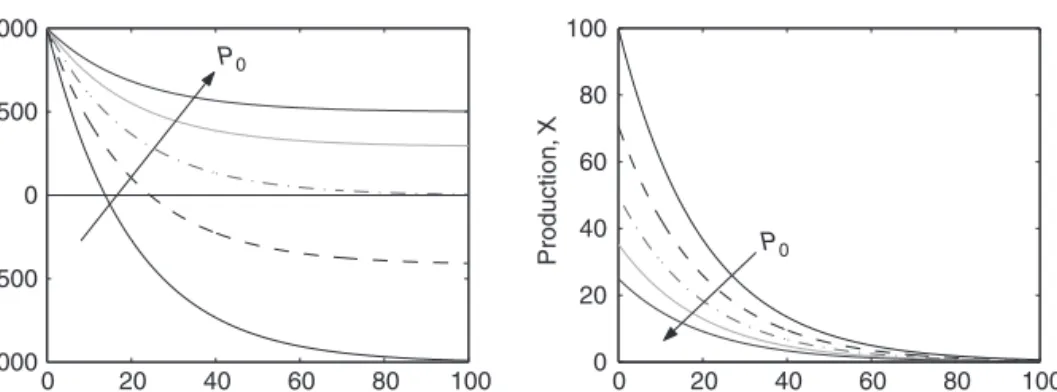
Figure 1.1. Five different depletion histories, identical except for initial price.P0 increases by factors of 2 in the direction of the arrows.
S0is presumed known;P0is not. IfP0is set too high, the demand will be stunted and the resource will go unutilized. IfP0is set too low, the demand will be too large and the resource will be depleted prematurely, leaving our mathematics of decision making invalid (Figure 1.1). The system is closed by invoking the Terminal Condition (TC): complete resource exhaustion as time goes to infinity:
S→0 ast→ ∞ (1.8)
Thus,
S0= a
P0ββr (1.9)
The initial price is thus
P0= a
S0βr 1β
(1.10) and the initial production rate is
X0= a
P0β =βrS0 (1.11)
IfP0is too high (X0too low), thenSis never exhausted. IfP0is too low (X0too high), then the resource is exhausted prematurely. In either case, production would be adjusted to satisfy the TC (Figure 1.2).
Rentis the integrated present worth of all net revenues:
R= ∞
0
e−rtX(t)P(t)dt (1.12) SinceP=P0ert, we have
R=P0
∞
0
X(t)dt=P0S0 (1.13)
0 20 40 60 80 100 0
200 400 600 800 1000
t
Storage, S
0 20 40 60 80 100
0 10 20 30 40 50
t
Production, X
0 20 40 60 80 100
0 2 4 6 8
10⫻104 ⫻104
t
Price, P
0 20 40 60 80 100
0 0.5 1 1.5 2 2.5 3
t
Revenue, PX
Figure 1.2. Exhaustion history that matches the TC. Demand isX =a/Pβ, with(a,β)=(100, 0.5).
For this simple case, the present worth of all future production is equal to today’s price times today’s total supply.
Program Oil1 illustrates the exhaustion history under these conditions. The 2 ODE’s are integrated forward in time with an explicit (Euler) forward-difference method. The initial price P0 needs to be adjusted manually to satisfy the TC.
Because numerical integration is not perfect, the relations developed above using the calculus correspond only approximately to the Oil1 simulation; the discrepancies vanish as the numerical timestep t becomes infinitesimally small.
1.1.2 Finite Demand
Next, add a ceiling priceP, which limits demand (Figure 1.3). Above this price, cus- tomers purchase a substitute product. The previous solution, in whichPrises without bound, is invalid. Equations 1.1–1.3 still govern, but the TC needs to be altered. The correct TC in this case is
S→0 asP→P (1.14)
1.1 Costless Production of a Sterile Resource 5
0 0.5 1 1.5
0 1 2 3 4 5
Production rate, X
0 0.5 1 1.5
0 1 2 3 4 5
0 0.5 1 1.5
0 1 2 3 4 5
Price, P
Production rate, X
0 0.5 1 1.5
– 2 –1 0 1 2 3
Price, P (a) (b)
(c) (d)
Figure 1.3. Four different demand functionsX(P). (a) base caseXa=P−β; (b) base case withP ≤P = 1; (c) linear demandXc =X0(1−P); (d) base case shifted,Xd+2=P−β. The dash lines indicate the continuation of the base case curve beyondX ≤0. Cases b, c, and d have finite demand.
which leads to exhaustion at finite timeT. From Equations 1.1 and 1.3, we have
P=P0erT (1.15)
S0= a P0ββr
1−e−βrT
(1.16) from which we obtain the final results
P0= a
βrS0+ a
Pβ β1
(1.17)
X0=βrS0+ a Pβ
(1.18)
T= 1 βrln
βrS0Pβ
a +1 (1.19)
These relations reduce to the previous ones asP→ ∞.
The above relations must govern at any time during the extraction history, else the trajectory would not be optimal and it would be altered, contrary to hypothesis.
Hence, we may drop the subscripts “0” and it is always true that
P= a
βrS+ a
Pβ β1
(1.20)
X =βrS+ a Pβ
(1.21)
T = 1 βrln
βrSPβ
a +1 (1.22)
withSthe remaining unexploited resource at any timetandP,X,Tthe contemporary price, production rate, and remaining time to exhaustion. Equations 1.20, 1.21, and 1.22 completely characterize the solution to Equations 1.1, 1.2, and 1.3, subject to the TC of exhaustion as price reaches the ceilingP.
ProgramOil1aillustrates these relationships. Figure 1.4 displays simulation results for finitePandT, achieved with the decision ruleX =X(S)(Equation 1.21).
Rent is, as above, the integrated present worth of all future production:
R= ∞
0
PXe−rtdt =P0 T
0
Xdt=P0S0 (1.23)
0 10 20 30 40 50
0 200 400 600 800 1000
t
Storage, S
0 10 20 30 40 50
0 10 20 30 40 50 60 70
t
Production, X
0 10 20 30 40 50
0 20 40 60 80 100
t
Price, P
0 10 20 30 40 50
0 200 400 600 800 1000
t
Revenue, PX
Figure 1.4. Extraction history with finite demand,Xa = 100P−β withP = 90 (case (b) in Figure 1.3).
This leads to exhaustion at finite time as shown.
1.1 Costless Production of a Sterile Resource 7
0 500 1000 1500 2000 0
10 20 30
S0 P0
10 20 30
0 500 1000 1500 2000 0
20 40 60 80 100
S0 X0
0 500 1000 1500 2000 0
20 40 60
S0
T
0 500 1000 1500 2000 0
2000 4000 6000
S0
R
Figure 1.5. P,X, andT as funtions of the total reserveS at any time (Equations 1.20–1.22). Demand:
X =aP−β;a=100;β=0.5;r=0.05;P=(10, 20, 30)as indicated by the linestyles.
This result is unchanged by the imposition of a ceiling price and the resultant finiteT.
SinceP0decreases asP decreases, ceiling price has the effect of diminishing overall rent, in accord with intuition.
Equations 1.20–1.22 giveP,X, andTas funtions of the total reserveSat any time, assuming complete exhaustion,X =aP−βandP≤P. Figure 1.5 plots these for three different values ofP. Rent peaks and begins to decline withSat high abundance in this scenario.
Consumers’ Surplus
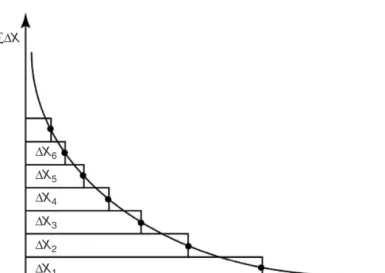
Consumption at pricePindicates a willingness to pay at leastP– that is, the value of the consumptionV ≥P. The consumer obtains a surplus equal to the difference V−P. Figure 1.6 illustrates a demand curve made up of individual usesX, each with its own valueV. If price is set atP, those users with higher value will purchase, and those with lower value will not. The consumers’ surplus (CS) is their accumulation:
CS=
(V −P)X (1.24)
for all increments where(V−P) >0. In the limit, CS(P)=
X(P)
0 (V −P)dx (1.25)
∆X6
∆X5
∆X4
∆X3
∆X2
∆X1
Value
∑∆X
Figure 1.6. Demand curve built up of individual incrementsX, ordered by decreasing individual value, plotted on the horizontal axis.
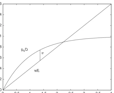
Value Rent
Consumers’ Surplus
P X
∑∆X
Figure 1.7. Demand curve as in Figure 1.6, adding the actual priceP. The area to the right of the price line is the consumers’ surplus; that to the left is the rent transferred to the seller.
Clearly, CS is a function ofP. Graphically, this is illustrated in Figure 1.7 as the area
“under the demand curve, to the right ofP”. The amountPXshown graphically is the total rent transferred to the seller. So transactions atPgenerate consumers’ surplus as well as rent.
Graphically, it is easy to see that an equivalent integral is CS(P)=
P
P
XdV (1.26)
An analogous concept of producers’ surplus (PS) divides the rent into production cost plus surplus: net rent. When production is costly, the producers’ surplus is the net rent.
1.1 Costless Production of a Sterile Resource 9
Consumers’ surplus is a static concept; time is fixed in its construction. Clearly in a depletion context, asPrises over time, CS will decrease: CS(P)=CS(P(t)). Suppose we have the base case demandX = aP−β, with a ceiling priceP. Then it is easy to verify that CS may be integrated to obtain
CS(P)= a 1−β
P1−β−P1−β
(1.27) The present worth of the consumers’ surplus is explored in Problem 34.
1.1.3 Linear Demand
As an extension of the preceding, consider the alternative demand function
P=P−bX (1.28)
We still have the requirement of exponential price growth
P=P0ert (1.29)
and thus
X = P−P0ert
b (1.30)
IntegratingdS/dt= −Xgives
S(t)=S0+1 b
P0
r (ert−1)−Pt
(1.31)
The Terminal Condition is
S(T)→0 asP(T)→P (1.32)
and therefore
P0erT =P (1.33)
rT =ln P
P0
(1.34)
and
S0= −1 b
P0
r (erT−1)−PT
(1.35)
0 20 40 60 80 0
0.2 0.4 0.6 0.8 1
S0 P0
Competitive
0 20 40 60 80
0 0.2 0.4 0.6 0.8 1
S0 X0
0 20 40 60 80
0 20 40 60 80 100
S0
T
0 20 40 60 80
0 1 2 3 4
S0
R
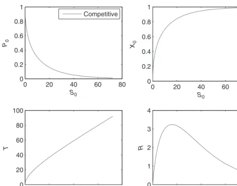
Figure 1.8. Optimal extraction relations for the linear demand case:r =0.05;P =1−X; competitive case.
A little rearrangement leads to
T= 1 r ln
P P0
(1.36)
S0= P br
P0
P −1+ln P
P0 (1.37)
X0= P−P0
b (1.38)
These last three equations relateS,X, andTtoP0; they comprise implicit functions X(S), T(S), andP0(S). There are no simple closed-form solutions, butX(S), T(S), andP0(S)can be evaluated numerically as inOil6M+C; the plots shown therein are reproduced in Figure 1.8. They characterize this system under linear demand, as did the closed-form Equations 1.20–1.22 for the earlier demand function.
As before, rentR = P0S0. It is interesting to note here that asSincreases, P0
ultimately decreases toward the limiting caseP0 → 0 asS → ∞. As a result, theR initially grows withSbut ultimately peaks and then decreases with increasingS. The point of maximum rent is found by settingdR/dt=0; the result is
ln
P P0
=2
1−P0
P
(1.39)
1.1 Costless Production of a Sterile Resource 11
There is one root of this equation in the range P0
P < 1: P0
P ∼0.2. The peak value ofSis
S∗= P br
1−P0
P
∼ P
br[.8] (1.40)
More resource beyond this limit results in less overall rent. Consumers’ surplus for this case is explored in Problem 35.
The programOil6M+Cprovides a simulation ofX,P,S, andRversus time.
1.1.4 Expanding Demand
Going back to the base case of an unbounded demand curve, Equation 1.2, consider the casea = a(t), an exogenous trend toward higher demand. This represents the same general price sensitivity, but growth inarepresents an outward shift in demand:
X = a(t)
Pβ (1.41)
This is illustrated in Figure 1.9. For example, a simple doubling of the number of resource-consuming machines would be expected to double the demand for the resource, all other things (includingP) being constant. Increasing the intrinsic use- per-machine would have the same effect. Growth inawould reflect the product of these two effects, extrinsic and intrinsic resource use or, equivalently, the resource intensity of individual use and the number of uses.
0 0.1 0.2 0.3 0.4 0.5 0.6 0.7
0 5 10 15 20 25 30 35 40
Price, P
Production rate, X
a(t)
Figure 1.9. Expanding demand curve, Equation 1.41, withβ=0.5.
As before we have
dS
dt = −X (1.42)
dP
dt =rP (1.43)
Integrating thePequation gives the price and production history:
P(t)=P0ert (1.44)
X(t)= a(t)
P0β e−βrt (1.45)
Exponential Demand Growth For this case,
a(t)=a0egt (1.46)
X(t)= a0
P0βe(g−βr)t=X0e(g−βr)t (1.47) Withg < βr, we have an unbounded future of finite production and the TC of resource exhaustion atT → ∞. Integrating gives us
S0= a0 P0β
1
βr−g = X0
βr−g (1.48)
and finally,
X0=(βr−g)S0 (1.49)
P0=
a0 (βr−g)S0
β1
(1.50) By comparison with the no-growth case, X is initially smaller and decays at the slower ratee(g−βr)t. Price is initially higher, and its growth rate is unchanged, ert. Rent= P0S0 is higher, proportional to P0. As the demand growth g approaches βr, pumping becomes infinitesimally small and nearly constant over time; price responds inversely and grows without bound. Forg > βr, the resource is never produced; the owner conserves in the face of rapidly escalating demand.
The case of declining demand (contraction) is the reverse:g<0. In this case,Xis initially larger than the constant-demand (g =0) reference case, and its decay rate is faster.
Linear Demand Growth
Next we examine the linear growth case
a(t)=ao+a1t (1.51)
1.1 Costless Production of a Sterile Resource 13
with exponential price growth
P=P0ert (1.52)
Production is again according to the demand curve
X =
ao+a1t
P0β e−βrt (1.53)
At long time,X →0; but early growth inXis possible. Differentiating, dX
dt = 1
P0β[a1−βr(a0+a1t)]e−βrt (1.54) This is positive att=0 when
a1>a0βr (1.55)
and if that is the case, there is a maximum inXatt∗: t∗= (a1−a0βr)
a1βr (1.56)
Fort>t∗, production declines toward zero atT → ∞. For exhaustion at that point, we require
S0= a0
P0ββr
1+ a1
a0βr
= X0
βr
1+ a1
a0βr
(1.57)
Equivalently,
X0= βrS0
1+aa01βr (1.58)
Compared with the no-growth case (a1 = 0), growth introduces a smaller initial production that peaks early, then decays to zero, asymptotically aste−βrt. (Small demand growth may not produce the peak.) Initial price is higher, growing at the rateert.
P0=
a0
1+aa0βr1 βrS0
β1
(1.59)
Rent is accordingly higher,P0S0.
Figure 1.10 illustrates the production history in this case, for peaking parameters a1>a0βr.
0 50 100 150 200 0
0.5 1 1.5 2 2.5
Time a(t)
X(t)
Figure 1.10. Time history of production with linear growth in demand. Parameters:a0=0.1;a1=0.01;
X0=1.;β=0.5;r=.05. Production peaks att∗=30.
Saturating Demand Growth
Consider the demand function in Equation 1.41 with a(t)=a0
1−e−st
(1.60) Demand is initially zero and rises toward the saturation levela0at the exponential rates. Again withP=P0ert, we have the production rate
X = a0
P0β
1−e−st
e−βrt (1.61)
and the reserve history
S(t)=S0− a0 P0β
1−e−βrt
βr −1−e−(s+βr)t
s+βr (1.62)
Applying the TC of complete exhausition ast→ ∞gives S0= a0
βrP0β s
s+βr
(1.63)
and Equations 1.61 and 1.62 for production and remaining stock become X(t)=S0
s+βr
s 1−e−st
e−βrt (1.64)
1.1 Costless Production of a Sterile Resource 15
S(t)=βrS0
s+βr
s 1−
βr s+βr
e−st
e−βrt (1.65)
Starting from zero, demand growth produces early growth in productionX, a peak at t∗, and a decline at the rateβronce demand has reached saturation ata0. The peak production occurs at
t∗=1 sln
s+βr βr
(1.66) In the limit of extremely fast saturation (very larges → ∞), we recover the base case: instantaneous onset of production, followed by monotonic decay (t∗ = 0) at the rate−βr. For intermediate saturation rates (s > βr), production at long time approaches the limiting relationX(t)=βrS(t), both decaying at the asymptotic rate βr. Essentially, at saturated demand we recover asymptotically the initial base case of constant demand.
When demand development is very slow, s < βr, then its development domi- nates production; but the peak production timet∗remains early and insensitive tos.
Expandingt∗in a Taylor series gives
t∗→ 1
βr (1.67)
This limit recovers the comparable result for linear demand growth, Equation 1.56, as it should.
Figure 1.11 illustrates the production history for demand saturating exponentially at a finite rate. Figure 1.12 illustrates the effect ofswith all other parameters constant, includingS0.
0 20 40 60 80 100 120 140 160 180 200
0 0.5 1 1.5 2 2.5
Time a(t)
X(t)
Figure 1.11. Time history of production with exponentially saturating growth in demand. Parameters:a0= 1;s=0.02;β=0.5;r=0.05. Peak production att∗=29.4.
0 20 40 60 80 100 120 140 160 180 200 0
2 4 6
Time s
Figure 1.12. Time history of production X for slow, intermediate, and fast growth saturation. Parameters:
a0=1;s =0.0002, 0.02, and 2.0;β=0.5;r =0.05; initial supply fixed atS0=170.
Note that this analysis requires knowledge from the beginning that demand will ultimately reacha0. That knowledge is embedded in the decision making.
Endogenous Demand Growth
It is interesting to speculate on what drives demand growth. We imagine a resource, like oil, which requires capitalization in combustion (fuels) and/or chemical manu- facturing (plastics) in order to be used; and these secondary products have their own consumer markets. In these cases, capital formation has an intrinsic lifetime of order 5–20 years (decay rateρ =0.05−0.20). So we speculate that the growth inawould be related to capital formation in the secondary industry:
da
dt +ρa=f(S,X,S/X,aS/X,P,π) (1.68) Increases inacould be driven by perception of large reservesS, large production X, large increases in reservesdS/dt, the exhaustion timescaleS/X, changes inPas a metric of scarcity, and/or the rate of rent formationπ. Clearly, the dynamics of the secondary industry, and their linkage to the primary resource industry, become critical here. This is beyond our scope.
1.2 DECISION RULES
The decision rule used so far has been dP
dt =rP (1.69)
withrthe interest rate applicable to investment of the proceeds of resource sale. This has been applicable to costless production in a competitive market. Three complica- tions need to be explored: taxation, the finite cost of production, and the possibility of monopoly production.
1.2 Decision Rules 17
1.2.1 Taxation
If we introduce a tax θ, we have a wedge between the price seen by the con- sumerP and the net rentP−θ accruing to the producer. Adapting the principle of intertemporal maximization of net rent (as used above), we have the decision rule
d(P−θ)
dt =r(P−θ) (1.70)
and
(P−θ)=(P0−θ)ert (1.71)
Two cases are interesting. First, consider a constant tax θ, which might be conceived as aconsumption tax. In this case, we have
P(t)=θ+(P0−θ)ert (1.72)
Withθ fixed, it loses relevance asPgrows. Consumption will be according to the demand function – for example,
X(t)= a Pβ =a
θ+(P0−θ)ert−β
(1.73) All other things remaining the same, initial priceP0will rise withθ, but it will not completely offset it; P0−θ will be less, so that initial net rent is less because ofθ.
This effect will be less pronounced as production proceeds; ultimately, growth inP overwhelms constantθ.
For example, for [S0,r,β,a,t]=[1000, 0.1, 0.5, 100, 0.5] and exhaustion att→ ∞:
for θ = 0, we find [P0,X0] = [4.4, 47.67]. The tax case θ = 2 gives [P0,X0] = [5.75, 41.70]. The early production is delayed by the imposition of the tax; later production is affected less. ProgramOil1-taxsimulates this.
A second case is aproportional tax,θ =τP. This amounts to a tax onrent, not on consumption per se. Following (1.70), we have
dP(1−τ)
dt =rP(1−τ) (1.74)
Withτconstant, the factor(1−τ)cancels, leavingP=P0ertand the whole production history unaffected byτ. The only effect is to redirect a portion of the rent,τR, to the public treasury, leaving the balance(1−τ)Rfor the original resource owner.
1.2.2 Costly Production
Again we generalize the concept of rent here as the present worth of resource sales minus expenses:
PX−CX (1.75)
wherePandX are the price and extraction rate as before andC is the unit cost of production. We will consider the case whereC depends on the remaining stock of resource, C = C(S). This would reflect the case where production becomes more costly as extraction proceeds, withCincreasing asSdecreases. The contributions to rentRfrom two adjacent production periods separated in time bytare
R=
[P1−C(S1)]X1+ 1
1+rt[P2−C(S2)]X2
(1.76) We wish to discover the effect of adjusting a hypothetical production pattern by moving a quantityof production forward in time, at the expense of later production, leaving all other things the same. We introduce the perturbations
X1= X2= − S1=0 S2= −·t
(1.77)
PerturbingRwith the changesXandS, we obtain R=
[P1−C(S1)]X1−X1dC
dSS1+ 1 1+rt
[P2−C(S2)]X2−X2dC dSS2
(1.78) With the perturbations above, we obtain
R=
[P1−C(S1)]− 1 1+rt
[P2−C(S2)]−X2dC dS·t
(1.79) The point of indifference to such an adjustment isR=0:
[P1−C(S1)]= 1 1+rt
[P2−C(S2)]−X2dC dSt
(1.80) Rearranging this, we obtain
[P2−C(S2)]=[1+rt] [P1−C(S1)]+X2dC
dSt (1.81)
and taking the limit ast→0, we have d(P−C)
dt =r(P−C)+XdC
dS (1.82)
Here we find two effects:
1. The rent rate (P−C), not price alone, must generally increase at the rate r with time.