Complex Functions Examples c-2: Analytic Functions - eBooks and textbooks from bookboon.com

Suppose that the function f(z) is analytic in a simply connected domain Ω (this roughly means that the domain contains no "holes"), then the value of the line integral. We have now exhausted all possibilities, so the open set system must consist of groups.

3 Complex Functions

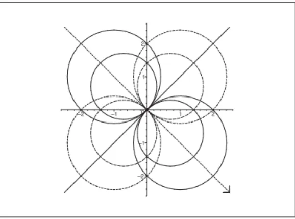
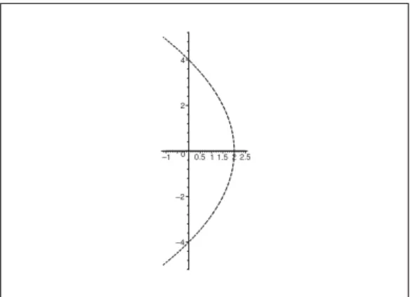
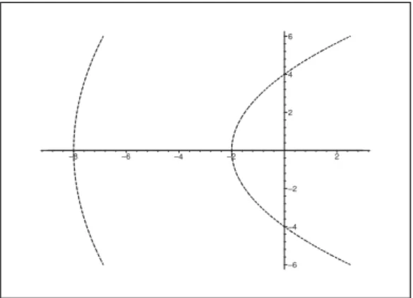
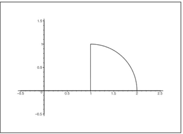
Finally, if we putz =iy (in Ω), then w=−2y2, y ∈R, which is a parametric description of the negative real axis, traverses twice. By a continuity argument (eg by puttingz= 12, which maps intow= 12), we conclude that the image is the interior of the parabola.

Figure 1: The domain Ω is the open parallel strip between the lines x = −1 and x = 1.

STUDY AT A TOP RANKED

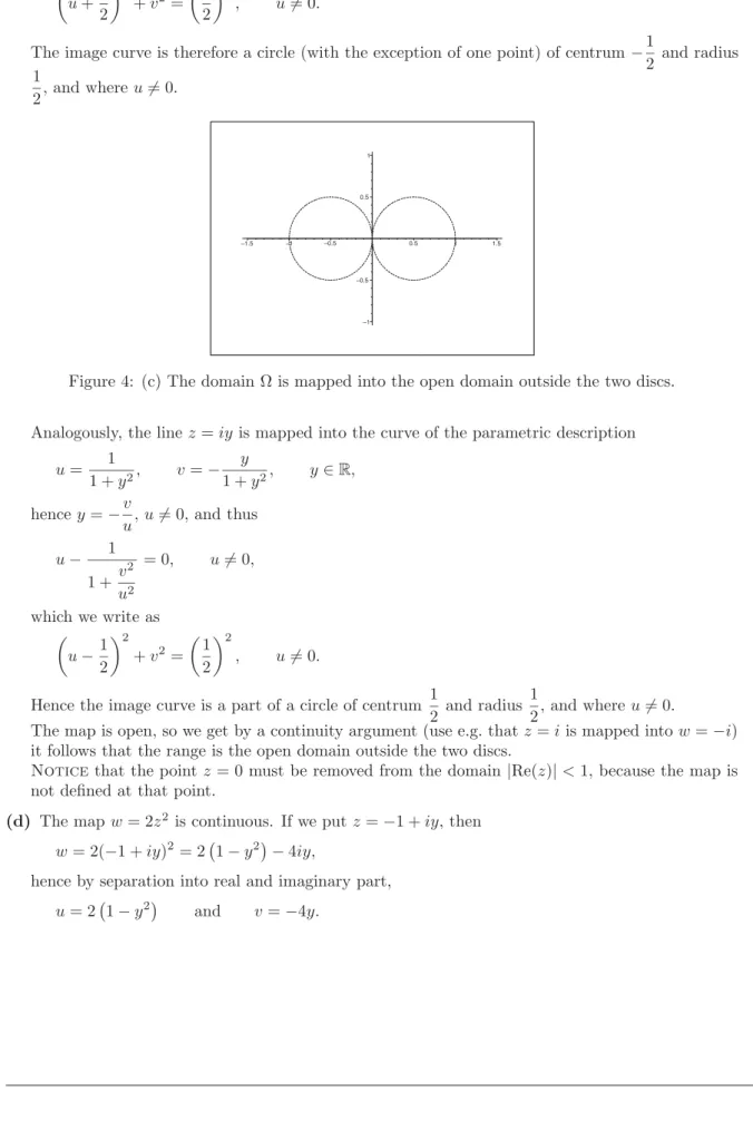
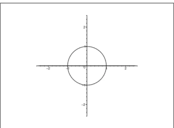
In summary, the range is that domain which "lies between" the circle and the straight vertical line = 1, so the range is a part of the open left half-plane given byu = 1, and which also lies outside the closed disc of the center. 1.

INTERNATIONAL BUSINESS SCHOOL

Click on the ad to read more Click on the ad to read more Click on the ad to read more Click on the ad to read more Click on the ad to read more Click on the ad to read more Click on the ad to read more Click on the ad to read more. Click on the ad to read more Click on the ad to read more Click on the ad to read more Click on the ad to read more Click on the ad to read more Click on the ad to read more Click on the ad to read more Click on the ad to read more Click on the ad to read more.

Figure 7: The domain Ω is the open parallel strip between the two horizontal lines.

CLICK HERE

Click on the ad to read more Click on the ad to read more Click on the ad to read more Click on the ad to read more Click on the ad to read more Click on the ad to read more Click on the ad to read more on the ad to read more Click on the ad to read more Click on the ad to read more. Click on the ad to read more Click on the ad to read more Click on the ad to read more Click on the ad to read more Click on the ad to read more Click on the ad to read more Click on the ad to read more on the ad to read more Click on the ad to read more Click on the ad to read more Click on the ad to read more.

Figure 15: (c) The image is the open complementary set of a disc w| > 1.

4 Limits

Example 4.4 Check whether limn→+∞zn exists for any of the following sequences (zn), and in case of existence, find the limit value. Click on the ad to read more Click on the ad to read more Click on the ad to read more Click on the ad to read more Click on the ad to read more Click on the ad to read more Click on the ad to read more Click on the ad to read more Click on the ad to read more Click on the ad to read more Click on the ad to read more Click on the ad to read more Click on the ad to read more. Click on the ad to read more Click on the ad to read more Click on the ad to read more Click on the ad to read more Click on the ad to read more Click on the ad to read more Click on the ad to read more Click on the ad to read more Click on the ad to read more Click on the ad to read more Click on the ad to read more Click on the ad to read more Click on the ad to read more Click on the ad to read more.

5 Line integrals

Click on the ad to read more Click on the ad to read more Click on the ad to read more Click on the ad to read more Click on the ad to read more Click on the ad to read more Click on ad to read more Click on ad to read more Click on ad to read more Click on ad to read more Click on ad to read more Click on ad to read more Click on ad to read more Click on the ad to read more Click on the ad to read more. Click on the ad to read more Click on the ad to read more Click on the ad to read more Click on the ad to read more Click on the ad to read more Click on the ad to read more Click on ad to read more Click on ad to read more Click on ad to read more Click on ad to read more Click on ad to read more Click on ad to read more Click on ad to read more Click on ad to read more Click on ad to read more Click on ad to read more Get help now. Click on the ad to read more Click on the ad to read more Click on the ad to read more Click on the ad to read more Click on the ad to read more Click on the ad to read more Click on ad to read more Click on ad to read more Click on ad to read more Click on ad to read more Click on ad to read more Click on ad to read more Click on ad to read more Click on the ad to read more Click on the ad to read more Click on the ad to read more Click on the ad to read more Click on the ad to read more.

Figure 28: The circle C with direction of circulation.

EXPERIENCE THE POWER OF FULL ENGAGEMENT…

Click on the ad to read more Click on the ad to read more Click on the ad to read more Click on the ad to read more Click on the ad to read more Click on the ad to read more Click on the ad to read more on the ad to read more Click on the ad to read more Click on the ad to read more Click on the ad to read more Click on the ad to read more Click on the ad to to read more Click on the ad to read more Click on the ad to read more Click on the ad to read more Click on the ad to read more Click on the ad to read more Click on the ad to read more read Click on the ad to read more.

Figure 43: The curve C 1 is composed of the quarter circle of radius A and centrum (1, 0) and the corresponding line segments to centrum.

SETASIGNThis e-book

6 Diﬀerentiable and analytic functions; Cauchy-Riemann’s equa- tions

On the other hand, the function is not continuous atz= 0, so it cannot be analytic either atz= 0. Click on the ad to read more Click on the ad to read more Click on the ad to read more Click on the ad to read more Click on the ad to read more Click on the ad to read more Click on the ad to read more Click on the ad to read more Click on the ad to read more Click on the ad to read more Click on the ad to read more Click on the ad to read more Click on the ad to read more Click on the ad to read more Click on the ad to read more Click on the ad to read more Click on the ad to read more Click on the ad to read more Click on the ad to read more Click on the ad to read more Click on the ad to read more. It follows from inspection that the Cauchy-Riemann equations are also satisfied at (0,0), so they lie over C.

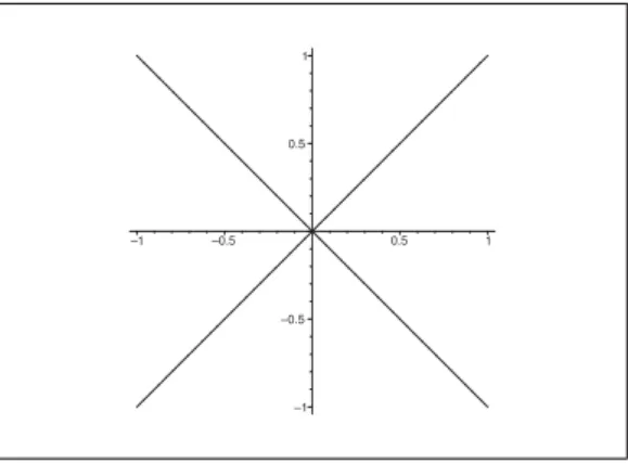
Click on the ad to read more Click on the ad to read more Click on the ad to read more Click on the ad to read more Click on the ad to read more Click on the ad to read more Click the ad to read more Click on the ad to read more Click on the ad to read more Click on the ad to read more Click on the ad to read more Click on the ad to read more Click on the ad to read more Click on the ad to read more Click on the ad to read more Click on the ad to read more Click on the ad to read more Click on the ad to read more Click on the ad to read more to read Click on the ad to read more Click on the ad to read more Click on the ad to read more. We see that one of the Cauchy-Riemann equations is satisfied, but the other. on the real axis, and the real axis does not contain an open domain of the plane.

Figure 44: The domain in (c) is the union of the two open angular sets which contain the positive and the negative real half axis, resp..

7 The polar Cauchy-Riemann’s equations

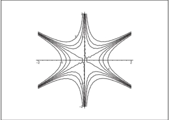
So the flow pattern does not change if we place barriers along these half lines. Click on the ad to read more Click on the ad to read more Click on the ad to read more Click on the ad to read more Click on the ad to read more Click on the ad to read more Click the ad to read more Click on the ad to read more Click on the ad to read more Click on the ad to read more Click on the ad to read more Click on the ad to read more Click on the ad to read more Click on the ad to read more Click on the ad to read more Click on the ad to read more Click on the ad to read more Click on the ad to read more Click on the ad to read more to read Click on the ad to read more Click on the ad to read more Click on the ad to read more Click on the ad to read more Click on the ad to read more Click on the ad to read more Click on the ad to read more Click on the ad to read more Click on the ad to read more Click on the ad to read more Click on the ad to read more Click on the ad to read more. On the other hand, it is easy to sketch the streamlines using MAPLE, and then we can use the equipotential curves to be orthogonal to this system of curves.

Figure 46: (a) The system of curves u(x, y) = c.

8 Cauchy’s Integral Theorem

9 Cauchy’s Integral Formula

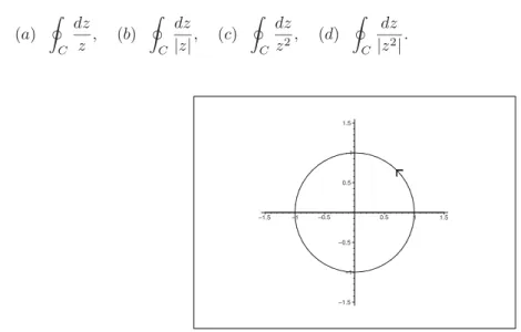
The smallest real number σ0, for which L{f}(z) is analytic in the half-plane Re(z)> σ0, is called the abscissa of convergence. Since integrandf(t)e−ztis continuous since the derivative with respect to the parameter z is continuous and absolutely integrable, it follows that L{f}(z) is continuously differentiable and its derivative is. We have used that the curve |z|= 4 is simple and closed and that the points −1 and 3 lie inside this curve.

10 Simple applications in Hydrodynamics

Furthermore, the orientation is indicated on the straight streamline, and the orientation generally follows continuity.