This Report Presented in Partial Fulfillment of the Requirements for the Degree of Bachelor of Science in Computer Science and Engineering.

(1)

PREDICTION OF TYPE 2 DIABETES USING DIFFERENT MACHINE LEARNING ALGORITHMS

BY

Tasmiah Rahman ID: 171-15-8805

Anamika Azad ID: 171-15-9057

This Report Presented in Partial Fulfillment of the Requirements for the Degree of Bachelor of Science in Computer Science and Engineering

^.

Supervised By Mr. Sheikh Abujar

Senior Lecturer Department of CSE

Daffodil International University

Co-Supervised By Md.Abbas Ali Khan

DAFFODIL INTERNATIONAL UNIVERSITY

DHAKA, BANGLADESH JANUARY 2021

(2)

APPROVAL

This Project titled “Prediction of Type 2 Diabetes Using Different Machine Learning Algorithms”, submitted by Tasmiah Rahman No:171-15-8805 and Anamika Azad, ID No:171-15-9057 to the Department of Computer Science and Engineering, Daffodil International University, has been accepted as satisfactory for the partial fulfillment of the requirements for the degree of B.Sc. in Computer Science and Engineering and approved as to its style and contents. The presentation has been held on Date: 28-01- 2021.

BOARDOFEXAMINERS

___________________________

Dr. Touhid Bhuiyan Professor and Head

Department of Computer Science and Engineering Faculty of Science & Information Technology Daffodil International University

Chairman

______________________

Abdus Sattar Assistant Professor

Internal Examiner

____________________________

Md. Jueal Mia Senior Lecturer

Internal Examiner

(3)

___________________________

Dr. Dewan Md. Farid Associate Professor

Department of Computer Science and Engineering United International University

External Examiner

(4)

DECLARATION

We hereby declare that, this project has been done by us under the supervision of Mr.

Sheikh Abujar, Senior Lecturer, Department of CSE Daffodil International University.

We also declare that neither this project nor any part of this project has been submitted elsewhere for award of any degree or diploma.

Supervised by:

Mr. Sheikh Abujar

Daffodil International University Co-Supervised by:

Md.Abbas Ali Khan Senior Lecturer Department of CSE

Daffodil International University Submitted by:

Tasmiah Rahman ID:171-15-8805 Department of CSE

Anamika Azad ID: 171-15-9057 Department of CSE

(5)

ACKNOWLEDGEMENT

First, we express our heartiest thanks and gratefulness to almighty God for His divine blessing makes us possible to complete the final year thesis successfully.

We really grateful and wish our profound our indebtedness to Mr. Sheikh Abujar, Senior Lecturer, Department of CSE Daffodil International University, Dhaka. Deep Knowledge

& keen interest of our supervisor in the field of “Data Mining and Machine Learning “to carry out this Thesis. His endless patience, scholarly guidance ,continual encouragement , constant and energetic supervision, constructive criticism, valuable advice ,reading many inferior draft and correcting them at all stage have made it possible to complete this thesis.

We would like to express our heartiest gratitude to Prof. Dr. Touhid Bhuiyan, Head, Department of CSE and Md. Abbas Ali Khan, Senior Lecturer, Department of CSE for their kind help to finish our thesis and also to other faculty member and the staff of CSE department of Daffodil International University.

We would like to thank our entire course mate in Daffodil International University, who took part in this discuss while completing the course work.

Finally, we must acknowledge with due respect the constant support and patients of our parents.

(6)

^ABSTRACT

Diabetes is a major threat for all over the world. It is rapidly getting worse day by day. It is a big challenge to determine diabetes properly and give proper treatment at a right time.

Now in this era of technology many machine learning algorithms are used to develop software to predict diabetes disease more accurately so that doctor can give patients proper advice and medicine which can reduce the risk of death. The purpose of this paper is to analyzing different Machine Learning algorithms for finding an efficient way to predict diabetes. In this thesis, we analyze 10 different machine learning algorithms which are Decision tree, Logistic regression, Multinomial Naïve Bayes, Gaussian Naïve Bayes, KNN, Support vector Classifier, Random Forest, Gradient Boosting, AdaBoost and Bagging by using a proper dataset. In our dataset there is 8 features and 2000 patients information. Here we find out the correlation of each attribute by using standard data mining technique. Dataset was preprocessed by using different preprocess method. We apply percentage split,10-fold and 15-fold cross validation technique on individual 10 different algorithms. In the end of our implementation, we find the highest accuracy in Decision tree which is 84.3% for percentage split,87% for 10-fold and 87.8% for 15-fold cross validation. Machine learning technique take less time for predict disease.

(7)

CHAPTER 4: EXPERIMENTAL RESULT AND

ANAYSIS 28-40

4.1 Introduction 28 4.2 Model Performance 28-38 4.2.1 Support Vector Machine (SVM)

4.2.2 Random Forest 4.2.3 Decision Tree 4.2.4 Logistic Regression 4.2.5 K-Nearest Neighbor 4.2.6 Multinomial Naïve Bayes 4.2.7 Gaussian Naïve Bayes 4.2.8 Gradient Boosting Classifier 4.2.9 AdaBoost Classifier

4.2.10 Bagging Classifier

4.3 Result Analysis 39 4.4 Summary 40

(10)

CHAPTER 5: CONCLUSION AND FUTURE

RESEARCH 41-42

5.1 Work flow of the Study 41

5.2 Conclusion 41-42 5.3 Limitations 42

5.4 Further Work 42

References 43

Plagiarism Report 44

(11)

List of the Figure

FIGURES PAGE NO

Figure 3.1: Experimental Work flow of the analysis 11

Figure 3.2: Sample of raw data 12

Figure 3.3: Distributed Target Variable 13

Figure 3.4: Frequency Distribution of each attribute 14

Figure 3.5: Heatmap of Correlation 15

Figure 3.6: Heatmap of missing value in dataset 16 Figure 3.7: Dataset after Handling Missing value 17

Figure 3.8: Decision Tree Important Features 18

Figure 3.9: Gradient Boosting Important Features 18

Figure 3.10: ROC Curve 26

Figure 3.11: Area under the ROC Curve (AUC) 27

Figure 4.1: ROC Curve for SVM 29

Figure 4.2: ROC Curve for Random Forest 30

Figure 4.3: ROC Curve for Decision Tree 31

Figure 4.4: ROC Curve for Logistic Regression 32

Figure 4.5: ROC Curve for K-Nearest Neighbor 33

Figure 4.6: ROC Curve for Multinomial NB 34

Figure 4.7: ROC Curve for Gaussian NB 35

Figure 4.8: ROC Curve for Gradient Boosting 36

Figure 4.9: ROC Curve for AdaBoost 37

Figure 4.10: ROC Curve for Bagging 38

Figure 4.11: Accuracy of all classifiers 39

(12)

List of the Tables

TABLES PAGE NO

Table 3.1: Confusion Matrix

19

Table 4.1: Accuracy Score for SVM 29

Table 4.2: Performance parameters for SVM 29

Table 4.3: Percentage Split for SVM 29

Table 4.4: Cross Validation (K=10) for SVM 29

Table 4.5: Cross Validation (K=15) for SVM 29

Table 4.6: Accuracy Score for Random Forest 30

Table 4.7: Performance parameters for Random Forest 30

Table 4.8: Percentage Split for Random Forest 30

Table 4.9: Cross Validation (K=10) for Random Forest 30

Table 4.10: Cross Validation (K=15) for Random Forest 30

Table 4.11: Accuracy Score for Decision Tree 31

Table 4.12: Performance parameters for Decision Tree 31

Table 4.13: Percentage Split for Decision Tree 31

Table 4.14: Cross Validation (K=10) for Decision Tree 31

Table 4.15: Cross Validation (K=15) for Decision Tree 31

Table 4.16: Accuracy Score for Logistic Regression 32

Table 4.17: Performance parameters for Logistic Regression 32

Table 4.18: Percentage Split for Logistic Regression 32

Table 4.19: Cross Validation (K=10) for Logistic Regression 32

Table 4.20: Cross Validation (K=15) for Logistic Regression 32

Table 4.21: Accuracy Score for K-Nearest Neighbor 33

Table 4.22: Performance parameters for K-Nearest Neighbor 33

Table 4.23: Percentage Split for K-Nearest Neighbor 33

Table 4.24: Cross Validation (K=10) for K-Nearest Neighbor 33

Table 4.25: Cross Validation (K=15) for K-Nearest Neighbor 33

Table 4.26: Accuracy Score for Multinomial NB 34

Table 4.27: Performance parameters for Multinomial NB 34

Table 4.28: Percentage Split for Multinomial NB 34

Table 4.29: Cross Validation (K=10) for Multinomial NB 34

(13)

Table 4.30: Cross Validation (K=15) for Multinomial NB 34

Table 4.31: Accuracy Score for Gaussian NB 35

Table 4.32: Performance parameters for Gaussian NB 35

Table 4.33: Percentage Split for Gaussian NB 35

Table 4.34: Cross Validation (K=10) for Gaussian NB 35

Table 4.35: Cross Validation (K=15) for Gaussian NB 35

Table 4.36: Accuracy Score for Gradient Boosting 36

Table 4.37: Performance parameters for Gradient Boosting 36

Table 4.38: Percentage Split for Gradient Boosting 36

Table 4.39: Cross Validation (K=10) for Gradient Boosting 36

Table 4.40: Cross Validation (K=15) for Gradient Boosting 36

Table 4.41: Accuracy Score for AdaBoost 37

Table 4.42: Performance parameters for AdaBoost 37

Table 4.43: Percentage Split for AdaBoost 37

Table 4.44: Cross Validation (K=10) for AdaBoost 37

Table 4.45: Cross Validation (K=15) for AdaBoost 37

Table 4.46: Accuracy Score for Bagging 38

Table 4.47: Performance parameters for Bagging 38

Table 4.48: Percentage Split for Bagging 38

Table 4.49: Cross Validation (K=10) for Bagging 38

Table 4.50: Cross Validation (K=15) for Bagging 38

(14)

CHAPTER 1 INTRODUCTION

1.1 Introduction

Diabetes mellitus which is commonly called diabetes is an incurable disease that occurs by metabolic disorder. It occurs because of pancreas unable to generate sufficient insulin or the human body unable to produce insulin to cells and tissues [1]. In Bangladesh, diabetes is one of the major cause of mortality. A large amount of people are affected by diabetes and die for it. Diabetes is not only a disease but also a creator of lot of disease. It harms heart, eyes, kidneys, nerves, blood vessels etc. Auto immune reaction, unhealthy lifestyle, unhealthy food habit, lack of exercise, fatness, environment pollution and genetic are mainly responsible in the sake of diabetes. Besides, there are a lot of reason to happen diabetes. The unplanned urbanization in Bangladesh is one of the premium reason. People cannot get enough places for culture like playing game and exercise. Moreover, people are eating junk food like pizza, burger and soft drinks which is full of sugar and fat. It would be consider as pre-diabetes if the fasting glucose level is between 100 mg/dl to 125 mg/dl.

And whereas the fasting glucose level is higher than 125 mg/dl, the person is diabetic otherwise it is normal [1].

The main three form of diabetes are:

Type 1 diabetes.

Type 2 diabetes.

Gestational diabetes

In this thesis, we are working along type 2 diabetes which is also known as hyperglycemia, Type 2 diabetes occurs whereas cells then tissue in the body cannot lead to insulin and it is also called non-insulin subordinate diabetes mellitus or adult starting diabetes [1].

Generally, it is found in people with high BMI and have inactive lifestyle.

(15)

Middle-aged people are more prone to diabetes. People who have type 2 diabetes they can make insulin but cannot use it properly.

Pancreas makes enough insulin and try to get glucose into cell but cannot do it and that’s why the glucose builds up in blood.

People who have type 2 diabetes are said to insulin resistance. Scientist have found several bits of gene that affect to make insulin. Extra weight or obese occurs insulin resistance. It can be define as metabolic disorder. When our digest system cannot work, it is responsible for type 2 diabetes.

1.2 Motivation

It is predicted that the number of Diabetes affected people will increment to 595 million by 2035.About 90% people are suffering in Type 2 diabetes. From recent work, it shows that diabetes is not dependent to age only. It dependent many other factors like insulin, BMI, Blood sugar level etc. Sometimes it faces some problem when people suffer more disease of the same category. In that time physicians are not able to determine this disease properly. For this concern in recent time machine learning techniques are used to develop software to help doctors for making decision of diabetes disease at a very early stage. Early stage predicting the probability of a person as the risk of diabetes can reduce the death rate.

Machine learning techniques are used medical dataset with multiple inputs and identify diseases more accurately in low cost.

1.3 Rational of the Study

As we know, all types of diabetes can create complication in our body and raise the risk of death. In 2014, globally 422 million affected by diabetes, the number of affected people will be about 642 million in 2040 [2].

1. Diabetes is a creator of different kind of disease. Diabetes leads to make complications including heart-attack, kidney damage, stroke, leg amputations and nerve damage. A patient of diabetes cannot heal the blow.

(16)

2. A person’s health becomes worse when he/she lives with diabetes and untreated. But the technology of early diagnosis like blood glucose measurement is now available in health care center.

3. Diabetes is very terrible illness in this current period. Every year about 1.6 million people died for diabetes [3].

4. There is a little possibility to affect by diabetes if diabetes belongs anyone’s family. But it does not mean that other person will be affected by diabetes if his/her close relative has diabetes. Though Type 2 diabetes mostly occurred by gene mutation.

5. The prevalence of Type 2 diabetes is increasing in short order in low and middle income countries because of increasing in the prevalence of obesity.

6. If diabetes could be detected and treated, people would live long and healthy.

1.4 Query of the Study

To improve our research we need some relevant question. The questions are:

1. What is diabetes prediction?

2. Can we make people sensible about diabetes?

3. How to gather data from dataset?

4. How to analysis and pre-process data?

5. Is the analysis appropriate or not?

6. How to get more accuracy?

7. Is the research relevant or not?

1.5 Prospective Outcome

In this part, we will discuss the expected result of our study that we want to achieve by following our plan.

1. Get good accuracy from applied algorithms.

2. To predict diabetes, want to focus on important factors.

3. Balance the outcome from several algorithm.

(17)

4. Make awareness about terrible circumstances of diabetes.

1.6 Report Layout

In this report firstly we have given a cover page with our title, supervisor name, and our group member name. Secondly, we have given the acknowledgement, abstract, list of contents, list of figures and list of table. Finally 5 separate chapter we have started to write.

Chapter 1 (Introduction) in this section we have discussed about introduction, motivation, rational of the study, query of the study, prospective outcome and report layout of this research work.

Chapter 2 (Background Instructions) in this section we have discussed about introduction, literature review, brief of the study, scope of the problem and challenges of this research work.

Chapter 3 (Overview of Methodology) in this section we have discussed about introduction, dataset description, implementation instrumentation, data visualization, correlation between features, data pre-processing, feature importance, train/test split, k- fold cross validation, model evaluation techniques, algorithm, roc curve and area under curve of this research work.

Chapter 4 (Experimental Result and Analysis) in this section we have discussed about introduction, model performance, result analysis and summary of this research work.

Chapter 5 (Conclusion, Limitation and Future Implication) in this section we have discussed about work flow of the study, conclusions, limitations and further work of this research work.

After that we have given the references that cooperates to complete the research work.

(18)

CHAPTER 2

BACKGROUND INSTRUCTION

2.1 Introduction

Diabetes is a common prolong disease and sometimes people did not realize how did they get it. And after that they do not understand what will happen next with them. Many types of ailments are created by diabetes such as complexity of vital organs and other organs of our body. If we can predict diabetes appropriately then it would be helpful to decrease diabetes because people will aware about it.

Type 1 diabetes happens when pancreas will not able to produce insulin. The insulin hormone balances our blood glucose. Type 1 diabetes mostly occurs because of abnormally blood sugar level. Lack of insulin in the blood then loss of insulin-producing beta cells in the pancreas are the primary reason of Type 1 diabetes [4]. It is also called insulin- subordinate diabetes mellitus [1].

May be you get type 1 diabetes by ancestral, if your parents has it. And it is most found in children. We can see the symptoms of Type 1 diabetes like thirst, tiredness, weight loss, frequent urination and increase in appetite in a diabetic person.

Type 2 diabetes mostly arrives when our body’s cells and tissues ineffectively respond to insulin and it is the most common diabetes in people. It is found that 90% people affected by Type 2 diabetes and 10% by Type 1 diabetes and gestational diabetes [5]. The body cannot use and make insulin because of high blood sugar. People who have Type 2 diabetes they take medicine to improve the body’s insulin and try to decrease the blood sugar of level which is produced by liver.

People with at any age, Type 2 diabetes can be arrived. But it is most commonly found in middle age or older people. Type 2 diabetes can be prolonged disease with other health ailment like heart disease, stroke, nerve damage, blindness, kidney damage and other part

(19)

of human body if blood sugar level is not adequately controlled through treatment.

Many types of hormones secrete during women pregnancy. Those hormones grow blood sugar level in the body and that’s why gestational diabetes occures. There is a possibility to occure type 2 diabetes and obesity later, who has gestation diabetes. Baby would die befor or after birth if gestation diabetes is untreated.

There is no clear pattern of inheritance of Type 2 diabetes. Hence, the awareness and drug can improve the health of people as well as there is no permanent cure for diabetes.

2.2 Literature Review

Diabetes prediction is the most researchable topic in machine learning. Most of the research work about predict diabetes has been done by several algorithm. Novel research works that related with our work will be discussed in this section.

In 2019, Neha Prerna Tigga and Shruti Garg they have utilized six meaching learning methods on PIMA Indian dataset and their own dataset. For the purpose of their research work RStudio was used for implementation and R programming language was used for coding. After that they have compared both datasets each other and got 94.10% accuracy from Random Forest Classifier [1].

In 2018, Han Wu, Shengqi Yang, Zhangqin Huang, Jian He and Xiaoyi Wang they aimed to improve accuracy of prediction and make a model that would be able to adaptive to more than one dataset. For this reason they used total three datasets and used WEKA toolkit for pre-processing, classifying, clustering, associating algorithms, and the visual interface. K- means cluster algorithm and logistic regression were used on data. They attained 95.42%

accuracy which is 3.04% higher than others [4].

In 2020, Md. Maniruzzaman, Md. Jahanur Rahman, Benojir Ahammed and Md. Menhazul Abedin, they have adopted four classifiers such as naïve bayes, decision tree, Adaboost and random forest and used diabetes dataset, conducted in 2009–2012. Their hypothesis

(20)

used LR-RF combination for feature selection technique which is machine learning based system and got 94.25% accuracy [2].

In 2019, Huma Naz and Sachin Ahuja approached deep learning to make a model for the risk measurement of diabetes in early stage. They have utilized total four diverse classifiers Artificial Neural Network, Naïve Bayes, Decision tree and Deep learning. For data preprocessing they have used sampling technique (linear sampling, shuffled sampling, stratified sampling, and automatic sampling) on the dataset. Deep learning gave the highest accuracy rate of 98.07% [3].

P. Moksha Sri Sai et al represented several algorithms like and K-Means Algorithm, Logistic Regression, Support Vector Machine, K-Nearest Neighbor (KNN), Random Forest, Decision Tree, Naive Bayes and show the performance between them. The study has discovered accuracy 93% in SVM which is highest accuracy [6].

Md. Kowsher et al presented a model by using scikit-learn which provides important tools for cleaning data, prepossessing data, and running classification algorithms. They applied seven different classifier and found highest accuracy in Random Forest which is 93.80%

[5].

M. M. Faniqul Islam et al utilizes three machine learning algorithm. After that they applied tenfold cross validation and percentage split evaluation technique and best result achieved by Random Forest which is 97.4% for 10-fold cross validation and 99% for percentage split method [7].

Mirza Shuja, Sonu Mittal and Majid Zaman they used Decision tree, Multi-Layer Perceptron, Simple Logistic, Support Vector Machines, and Bagging in two phases for reducing data imbalance. They obtained desired result from one phase with SMOTE and Decision tree. The accuracy is 94.70% [8].

(21)

Wenqian Chen et al proposed a hybrid prediction model by K-means and Decision tree algorithms. And they found the best accuracy from that hybrid prediction model than other classification models. The accuracy is 90.04% [9].

Dr. D. Asir Antony Gnana Singh, Dr. E. Jebamalar Leavline and B. Shanawaz Baig presented a diabetes prediction system to diagnosis diabetes using medical data. They applied Naïve Bayes, Multilayer Perceptron and Random Forest machine learning algorithm and k-fold cross validation, percentage split and use training dataset with preprocessing technique and without preprocessing technique. The pre-processing technique conducts better average accuracy for NB [10].

Deepti Sisodia and Dilip Singh Sisodia they have experimented to predict the possibility of diabetes at early stage. They utilized three machine learning algorithm Decision Tree, Support Vector Machine and Naïve Bayes. And earned good accuracy of 76.30% by Naïve Bayes and verified by ROC curve [11].

2.3 Brief of the Study

From the previous literature research and study we have known that there are so many work in this bounds. And the research succeed in their own way. Our research work also a little bit similar with previous study some way. We have worked with two thousands data. There are nine attributes in the dataset. Then we have pre-processed data by using difference preprocessing technique. After that we have utilized 10 algorithm such as SVM, Decision tree, Logistic regression, Naïve Bayes, KNN and Random Forest etc. And finally we have earned good result from the work. Though we have observed there is no real implementation as people are comfortable with doctor for consultation. But people would rely on this computerized diabetes prediction as they consult with doctor if it works appropriately.

(22)

2.4 Scope of the problem

As our research work is about prediction diabetes and it is one of the most significant and unique work of medical area. The aim of our hypothesis will give a better prediction about diabetes. People will get a clear idea about diabetes from our research work and take action to reduce the risk of this disease.

2.5 Challenges

As we are beginner in this sector so face many difficulties to reach our expected goal. The initial challenge which we face in this thesis to collect data. Because nobody wants to give their data without reference. Another challenge we face to preprocess data. We also face difficulties for choosing the perfect Algorithm which will give us good accuracy in diabetes prediction.

(23)

CHAPTER 3

OVERVIEW OF METHODOLOGY

3.1 Introduction

In this chapter, we will discuss about the working procedure that we follow to find the expected result in our thesis. All research work has its own strategy to solve the problem.

Machine learning is a subset of Artificial intelligence. It is an area of Computer Science that use several statistical methods and analyzing data, process data and find a useful pattern between data and make different pattern to achieve the expected goal. It teaches a computer so that the computer gains the ability to learning data, making decision, thinking capability without human interaction. It is able to predict accurate prediction when data is given in a computer system.

Generally, there are two main categories of machine learning algorithms they are supervised and unsupervised learning. Supervised learning uses labeled dataset. At first it uses a large portion of data to train algorithms. This data set called training dataset. After training the model it has the ability to predict output properly. For disease prediction problem supervised learning process is used significantly. Unsupervised learning is a process that work with unlabeled data. It creates some cluster of the data with same characteristic.

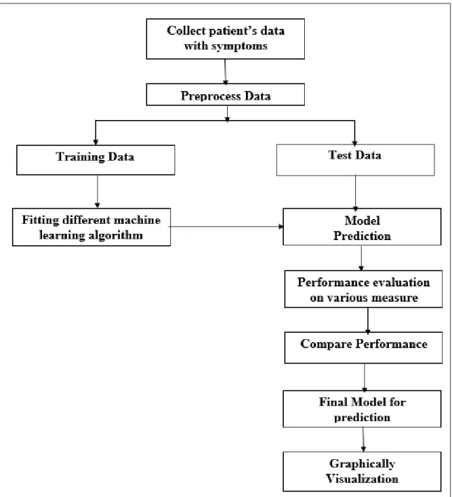
The number of diabetes patient is increasing at an alarming rate all over the world. In this research work we tried to predict diabetes disease at a very early stage. we use supervised learning process in this thesis. So that at first, we split our data set into two parts. Training data for trained the model and testing data for measure how accurately the model can predict the disease. We apply several machine learning algorithms, different data preprocessing technique for predict the diabetes disease more accurately.

(24)

The model of this research work is given below:

Figure 3.1: Experimental Work flow of the analysis

(25)

3.2 Dataset Description

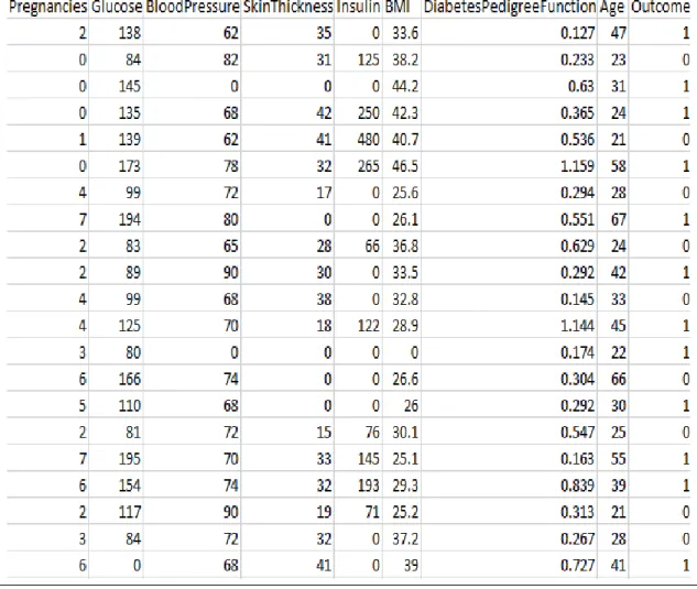
Data description can define as where all the information of data is sorted in a data set and user can easily understand and use that data. Our data set consists of 9 columns and 2000 rows. Here first 8 columns are considered as feature which is used for predict last column

“Outcome” that define the patients has diabetes or not. Here 0 means not affected by diabetes and 1 means affected by diabetes. The data set is based on female data. 2000 rows in dataset means there is 2000 patients’ information provided in this data set.

Figure 3.2: Sample of raw data

(26)

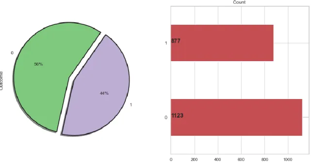
Figure 3.3: Distributed Target Variable

In Figure 3.3 we distributed the target variable “Outcome “where we see that 877 patients have diabetes disease and 1123 patients have no diabetics in our dataset.

3.3 Implementation Instrumentation

To complete this study and develop the model we have used some hardware instrument and software instrument. Those are

Software:

Anaconda: Anaconda is a software that utilized the idea of making environment. It is an allocation of Python and full of hundreds of packages related to scientific programming, data science, development and more.

Microsoft Excel Worksheet: We have converted the data set from (.csv) format to excel format by using and used Microsoft Excel Worksheet for data entry. Then we have put the data set into Anaconda for implementation.

Hardware: Key-board, mouse and laptop.

Data Set: For the purpose of our study, we have collected this dataset from different online sources.

(27)

3.4 Data Visualization

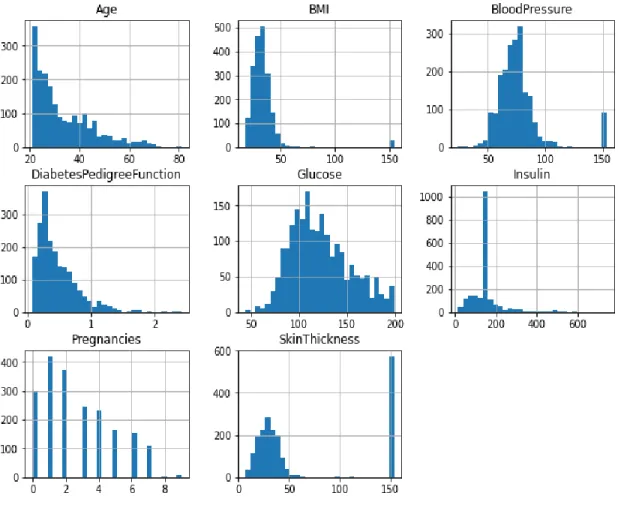
Data visualization help us to understanding data clearly, make the best decision among several decision to solve problem and comparative analysis. In figure 3.4 shown the frequency distribution of our dataset. Frequency distribution is a statistical method, where we can understand the observation number within a given interval. Here we visualize each feature by histogram. Histogram is a graphical display of distribution numerical data. Here y axis represents the count of frequency and x axis represent the feature that we want to be measured. From visualization of frequency distribution anyone can easily understand the majority occurrence range in the dataset.

Figure 3.4: Frequency Distribution of each attribute

(28)

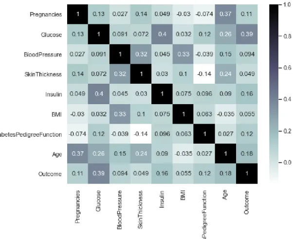
3.5 Correlation between features

In this figure 3.5 we see the correlation between every two columns in our data set. Here the right-hand side of the figure is shown the value of correlation that has marked two different color. The lighter side means less correlation and the darker side means strong correlation between them. Here, if we considered the dependent column “Outcome” we can find out the correlation of “Outcome” column with all other columns. From “Outcome”

column we see that “Outcome” is less dependent on “BloodPressure” and “Glucose” is very important column for predicting diabetes disease. If we want to drop any column, we can drop the “BloodPressure” Column form our dataset.

Figure 3.5 Heatmap of Correlation

(29)

3.6 Data Pre-Processing

It is not possible to get an organized data from real world. In Real world most of the time the dataset is incompatible, lack of particular important behavior and contain many errors.

Data preprocessing is a technique to reduce this problem. Data Preprocessing is very important for data set. It can prepare the raw data for making it suitable to build different machine learning model. We notice there is lots of missing value in different columns in our data set. Before use this dataset, we handle the missing value by using different statistical method. It can prevent the loss of data.

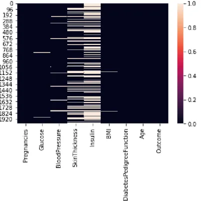
3.6.1 Missing value visualization

In figure 3.6 shows visualization of the missing value in our dataset. Here the darker side indicate no missing value and lighter side indicate the presence of missing value in specific column. From the figure, we notice that there are lots of missing value in our dataset.

Before applying different machine learning algorithm in this dataset, we need to handle this missing value for finding better performance.

Figure 3.6: Heatmap of missing value in dataset

(30)

3.6.2 Handling Missing value

From figure 3.6 we notice that there are many missing values in several column in our dataset. Before utilize this dataset at first, we need to handle the missing value by using statistical method. Here in our thesis, we replaced that missing value with the mean value of that column. Replacing the missing value with the mean value is a statistical method for handling missing value.

Figure 3.7: Dataset after Handling Missing value

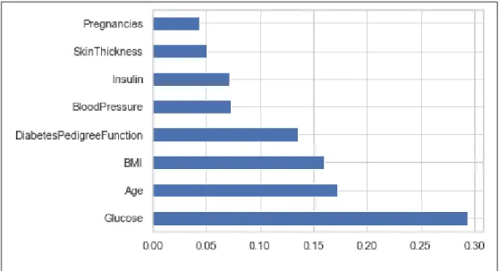
3.7 Feature Importance

Sometimes working with lots of features reduce the accuracy of the model. So, we need to work with important features. Feature importance means which features in the dataset are most important for predicting accuracy in a certain model. Some feature doesn’t affect the

(31)

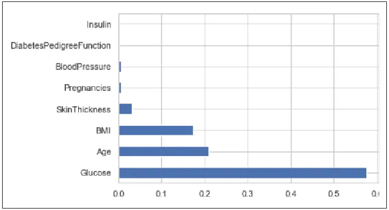
accuracy. In figure 3.8 and 3.9 are shown the important features for Decision tree and Gradient Boosting Algorithm respectively. Here we notice that different accuracy in every column for different algorithm.

Figure 3.8: Decision Tree Important Features

Figure 3.9: Gradient Boosting Algorithms Important Features

(32)

3.8 Train/Test Split

Train/Test split method means when the dataset is divided into two-part that is training data set and testing data set. Training data set used for train the model and the test data set is used for determine the prediction from the model that is already trained by training data set. Large portion of data is used for trained the model.

3.9 K-fold Cross Validation

K fold cross validation is a technique when we divided the data set into k subsets. Here we used one set for testing data set and (k-1) sets for training data set. This process is done repeatedly for k times for each subset being the test set. Then the final result is found by averaging of k result. This process is applying to predict best outcome for disease prediction. Basically, it is used when data is limited. We use this method in our data set. In this thesis work we use the value of k is 10 and 15.

3.10 Model Evaluation Techniques

By applying different performance parameter, we can evaluate the performance of Machine learning algorithm which we applied in this thesis work.

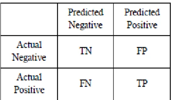
3.10.1 Confusion Matrix

Confusion matrix is a two-by-two matrix that regulates the performance of a classification model. There can be 4 cases from where we know about the number of positive and negative occurrences were classified correctly or incorrectly. The rows of a confusion matrix illustrate actual class and the columns of a confusion matrix illustrate predicted class. Table 3.1 presents a confusion matrix.

(33)

Table 3.1:Confusion Matrix

True Positive (TP): True Positive means both actual class and predicted class is true (1) so, patient has complexity in reality and also classified true by the model.

True Negative (TN): True Negative means both actual class and predicted class is false (0) so, patient has not complexity in reality and also classified false by the model.

False Positive (FP): False Positive means actual class is false (0) but predicted class is true (1) so, patient has not complexity in reality but classified true by the model.

False Negative (FN): False Negative means actual class is true (1) but predicted class is false (0) so, patient has complexity in reality but classified false by the model.

3.10.2 Accuracy (ACC)

Accuracy is measured by total number of correct classifications divided by total number of classifications. The formula is presented by,

𝒂𝒄𝒄𝒖𝒓𝒂𝒄𝒚 = 𝑻𝑷 + 𝑻𝑵

𝑻𝑷 + 𝑭𝑷 + 𝑻𝑵 + 𝑭𝑵 (𝟏)

3.10.3 Precision

Precision is measured by true positive divided by total number of predicted yes. The formula is presented by,

𝒑𝒓𝒆𝒄𝒊𝒔𝒊𝒐𝒏 = 𝑻𝑷

𝑻𝑷 + 𝑭𝑷 (𝟐)

(34)

3.10.4 Recall / Sensitivity

Recall is measured true positive divided by total number of actual yes. The formula is presented by,

𝒓𝒆𝒄𝒂𝒍𝒍 = 𝑻𝑷

𝑻𝑷 + 𝑭𝑵 (𝟑)

3.10.5 Specificity

Specificity is measured by true negative divided by total number of actual negative. The formula is presented by,

𝒔𝒑𝒆𝒄𝒊𝒇𝒊𝒄𝒊𝒕𝒚 = 𝑻𝑵

𝑻𝑵 + 𝑭𝑷 (𝟒)

3.10.6 F1 Score

F1 Score is measured by multiplication of precision and recall divided by addition of precision and recall and multiply by 2. The formula is presented by,

𝑭𝟏 = 𝟐 ∗ 𝒑𝒓𝒆𝒄𝒊𝒔𝒊𝒐𝒏 ∗ 𝒓𝒆𝒄𝒂𝒍𝒍

𝒑𝒓𝒆𝒄𝒊𝒔𝒊𝒐𝒏 + 𝒓𝒆𝒄𝒂𝒍𝒍 (𝟓)

3.10.7 Matthews Correlation Coefficient (MCC):

In machine learning we can evaluate the quality of binary classifications by using MCC. It is a reliable statistical rate and gives great result for imbalanced dataset. The score of MCC is between -1 to +1. The equation of MCC is presented by,

𝑴𝑪𝑪 = (𝑻𝑷 ∗ 𝑻𝑵) − (𝑭𝑵 ∗ 𝑭𝑷)

√(𝑻𝑷 + 𝑭𝑵) ∗ (𝑻𝑵 + 𝑭𝑷) ∗ (𝑻𝑷 + 𝑭𝑷) ∗ (𝑻𝑵 + 𝑭𝑵) (𝟔)

3.11 Algorithms:

We use different machine learning algorithms in our thesis for prediction accuracy. In this work we tried to find out the number of patients those have diabetes disease and the number

(35)

of patients those are not affected by diabetes. For this reason, we are applied 12 different algorithms in this dataset. These 10 algorithms are Logistic Regression, Support Vector Machines (SVM), Gaussian Naïve Bayes, Multinomial Naïve Bayes, Decision Tree, Random Forest, Bagging, Ada-Boost, Gradient Boosting and K-Nearest Neighbor. We will compare these algorithms based on different parameter. After comparing these algorithms, we will find the best algorithm that can predict the output more accurately.

3.11.1 Logistic Regression

Logistic Regression is a classification algorithm of supervised learning which deals with probability to predict an outcome for dependent variable which is binary nature by using logistic function. It works with continuous and discrete value and its goal to find the best fitting model for independent and dependent variable relationship. In a graph we found it like S shape. Which means there is no chance that the value would be fraction, so the value would be either 0 or 1. And it never crosses the limit. It maintains any relationship. The formula of Logistic Regression is,

𝒇(𝒙) = 𝟏

𝟏 + 𝒆^−𝒙 (𝟕)

3.11.2 Support Vector Machines (SVM)

Support Vector Machines is a supervised learning algorithm which is used for recognized sample with training data which is labeled format by a separating hyperplane. Vector means training example by construct some machine or classifier. For linear classifier, SVM use subset of training data and it is used to represent decision boundary. The hyperplane depends of maximum width of margin so you have to choose most optimal one hyperplane.

It is not equally performed well on any unseen example. The formula of SVM is presented by,

𝐠(𝐱) = 𝒘^𝑻𝒙 + 𝒃 (𝟖)

(36)

3.11.3 Gaussian Naïve Bayes

Gaussian Naïve Bayes is a form of Naïve Bayes and Probabilistic approach algorithm. It is utilized for continuous values. Firstly, the algorithm starts classification after that total block come. It is based on Gaussian distribution where the data is lied between a center point that means they will not very right or left. The formula is given below,

𝑷(𝒙_𝒊|𝒚) = 𝟏

√𝟐𝝅𝝈_𝒚^𝟐

𝐞𝐱 𝐩 (−(𝒙_𝒊− 𝝁_𝒚)^𝟐

𝟐𝝈_𝒚^𝟐 ) (𝟗)

This function is called probability density function. Here, we can search out mean, variance and standard deviation together.

3.11.4 Multinomial Naïve Bayes

Multinomial Naïve Bayes is also a form of Naïve Bayes and it is utilized for combined probability. It is fit with discrete count features which is in a form of binary. Either we will get 0 or 1. Multinomial classification is simply the case when we have more than 2 classes.

It is based on Multinomial distribution means it has generalization of binary distribution where there are two or more mutually outcomes of a trial. The formula is,

𝑷(𝒄|𝒙) =𝑷(𝒙|𝒄)𝑷(𝒄)

𝑷(𝒙) (𝟏𝟎) 3.11.5 Decision Tree

Decision Tree is a nothing but a tree structured classifier that used on concept of classification and concept of regression. When an input comes in the model, decision tree shows the class of that particular input. The significance of decision nodes is nothing but test. Test is performed on the attribute. To make a decision tree we need a dataset. Then we have to calculate the entropy of target value and predictor attribute value. Then we will

(37)

gather information of all attribute and finally which attribute has more information it would be root node. In this way data would be split and we will get our decision tree and could be able to make decision.

3.11.6 Random Forest (Ensemble)

Random forest is kind of a powerful and popular ensemble classifier which is using decision tree algorithm in a randomize way. It is combined of multiple decision tree. To build every single decision tree it uses bagging technique. When we classify a new object, we got classification from each tree as tree vote. And the major vote for classification is accepted. That is why it rather provides more accurate result than single decision tree. And in the case of regression takes the average of the outputs by different trees.

3.11.7 Bagging

Bagging other name Bootstrap aggregation which is meta-algorithm for machine learning ensemble that taking sample with replacement. It is used different subset of data and same model which is known as base estimator. If we use Decision Tree as a model in Bagging then it will be Random Forest. By using bagging, it is possible to decrease variance of a model by generating additional test data. Once the size of dataset is increased, we can tune the model to be more immune to variance. The formula is presented by,

𝐟(𝐱) = 𝟏

𝑩∑ 𝒇_𝒃(𝒙) (𝟏𝟏)

𝑩

𝒃=𝟏

3.11.8 Ada-Boost

Ada-boost is known as sequential learning method. It is also decreasing the variance of decision trees on binary classification issues. This learning can detect the complex problem that previous learning cannot detect by errors. Here learning is happening with weight

(38)

updating. When a model does misclassification then we increase weight and when does right classification we decrease weight. And it will be running until the error becomes 0.

Ada-boost used decision stump for every base estimator in depth 1. The formula can be represented by,

𝑭(𝒙) = 𝐬𝐢𝐧( ∑ 𝜽_𝒎𝒇_𝒎(𝒙)) (𝟏𝟐)

𝑴

𝒎=𝟏

3.11.9 Gradient Boosting

Gradient boosting is a type of boosting technique that works on reducing error sequentially.

It can be used for any loss function. It is trying to build new sequential models for fit data, that data which is giving error. Here learning is happing by optimizing the loss function (actual-predicted). Gradient boosting used two type of base estimators, first is average type of model and second is decision tree with having the full depth.

3.11.10 K-Nearest Neighbor

K-Nearest Neighbor is considered as supervised machine learning algorithm that can able to find out the classification and regression using numbers (K) neighbors. K would be integer number. To execute KNN, first we need a categorical dataset. Then the value of K will be defined as odd number. Next calculate the distance of new instance from nearest neighbor. Finally, new instance would assign in majority of neighbor class. It works with either Euclidean distance or Manhattan distance with neighbor vote.

(39)

3.11 ROC Curve

ROC means Receiver operating characteristic. It is a graphical plot of True Positive Rate against False Positive Rate or we can say a comparison of sensitivity and (1-specificity). It measures different thresholds value for determine the best threshold point of the model.

Form ROC curve we understand how good the model for predicting positive and negative class.

Figure 3.10: ROC Curve

(40)

3.13 Area Under Curve (AUC):

AUC is the area under ROC curve. This is use for determine the performance of the classifier. Its range is 0 to 1. The higher value of AUC means better performance 0.5 means the model has no separation capacity. For balanced dataset, AUC are useful for measure the performance. Higher value defines better performance. In figure 3.5 shown the ROC curve and the shade under ROC curve is AUC. Here false positive rate is plotted on X-axis and True positive Rate is plotted on Y axis.

Figure 3.11: Area under the ROC Curve (AUC)[12]

(41)

CHAPTER 4

EXPERIMENTAL RESULTS AND ANALYSIS

4.1 Introduction:

In this chapter we will discuss about our experimental result that we found after implementing different machine learning algorithm in this system. For implementation we divide our data set into two parts, training dataset and testing dataset. Here we use 70%

data as a training dataset and 30% data for test data set. We also apply cross validation method for finding better performance. At first, we trained our training dataset by using different machine learning algorithm and build a model then we tested on test dataset in this model. We compare the result with different classifier performance.

4.2 Model Performance:

The expected outcome of this research has been found by applying different machine learning algorithm. Here we use 10 different machine learning algorithms. We use both cross validation and percentage split technique then we compare the algorithm for find out the best algorithm from which we can obtain the highest accuracy. For measure the performance of each model we built confusion matrix for both k fold cross validation and percentage split method. Where k means the dataset is split into k number of groups. Here we assume k=10 and k=15-fold cross validation. Confusion matrix has four parts True Positive (TP), True Negative (TN), False Positive (FP), False Negative (FN). Form this value we find the Accuracy, Precision, Recall, F1-Score, MCC score and AUC score to measure the performance of every machine learning algorithm. For each algorithm Performance Parameter, confusion matrix and ROC curve is shown below.

(42)

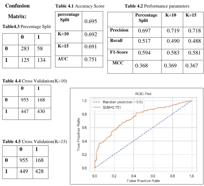
4.2.1 Support Vector Classifier (SVC):

After applying Support Vector machine algorithm, we found the confusion matrix for both percentage split and k fold cross validation method. Where k is 15 and 10. From confusion matrix we calculate Precision, Recall, Accuracy, MCC score and F1-Score for both percentage split and cross validation method and also measure AUC score. ROC curve represents the AUC of the algorithm in the figure.

Confusion

Table 4.1 Accuracy Score Table 4.2 Performance parameters

Matrix:

Table4.3 Percentage Split

Table 4.4 Cross Validation(K=10)

Figure 4.1 ROC Curve for SVM

0 1

0 283 58 1 125 134

percentage

Split 0.695

K=10 0.692

K=15 0.691

AUC 0.751

Percentage Split

K=10 K=15 Precision 0.697 0.719 0.718

Recall 0.517 0.490 0.488

F1-Score MCC

0.594 0.368

0.583 0.369

0.581 0.367

0 1

0 955 168

1 447 430

0 1

0 955 168 1 449 428

(43)

4.2.2 Random Forest Classifier:

After applying Random Forest Classifier algorithm, we found the confusion matrix for both percentage split and k fold cross validation method. Where k is 15 and 10. From confusion matrix we calculate Precision, Recall, Accuracy, MCC score and F1-Score for both percentage split and cross validation method and also measure AUC score. ROC curve represent the AUC of the algorithm in the figure.

Confusion Table 4.6 Accuracy Score Table 4.7 Performanceparameters

Matrix:

Table4.8Percentage Split

Figure 4.2 ROC Curve for Random Forest

Split

K=10 K=15 Precision 0.781 0.832 0.833

Recall 0.772 0.814 0.825

0.776 0.649

0.823 0.696

0.829 0.705

Percentage

Split 0.808

K=10 0.858

K=15 0.855

AUC 0.870

0 1

0 285 56 1 59 200

0 1

0 979 144 1 163 714

0 1

0 978 145 1 153 724

(44)

4.2.3 Decision Tree Classifier:

After applying Decision Tree Classifier algorithm, we found the confusion matrix for both percentage split and k fold cross validation method. Where k is 15 and 10. From confusion matrix we calculate Precision, Recall, Accuracy, MCC score and F1-Score for both percentage split and cross validation method and also measure AUC score. ROC curve represent the AUC of the algorithm in the figure.

Confusion Table 4.11 Accuracy Score Table 4.12 Performanceparameters

Matrix:

Figure 4.3 ROC Curve for Decision Tree

Split 0.843

K=10 0.870

K=15 0.878

AUC 0.851

K=10 K=15 Precision 0.811 0.890 0.897

Recall 0.830 0.806 0.810

0.820 0.674

0.846 0.742

0.852 0.747

0 1

0 291 50

1 44 215

0 1

0 1036 87

1 170 707

0 1

0 1042 81

1 166 711

(45)

4.2.4 Logistic Regression:

After applying Logistic Regression algorithm, we found the confusion matrix for both percentage split and k fold cross validation method. Where k is 15 and 10. From confusion matrix we calculate Precision, Recall, Accuracy, MCC score and F1-Score for both percentage split and cross validation method and also measure AUC score. ROC curve represent the AUC of the algorithm in the figure.

Confusion Table 4.16 Accuracy Score Table 4.17 Performance parameters

Matrix:

Figure 4.4 ROC Curve for Logistic Regression

Split

0.686

K=10 0.682

K=15 0.684

AUC 0.726

K=10 K=15

Precision 0.660 0.671 0.672

Recall 0.563 0.540 0.545

F1-Score

MCC

0.608

0.352

0.598

0.346

0.602

0.349

0 1

0 266 75 1 113 146

0 1

0 891 232 1 403 474

0 1

0 890 233 1 399 478

(46)

4.2.5 K-Nearest Neighbors Classifier:

After applying K-Nearest Neighbors Classifier algorithm, we found the confusion matrix for both percentage split and k fold cross validation method. Where k is 15 and 10. From confusion matrix we calculate Precision, Recall, Accuracy, MCC Score and F1-Score for both percentage split and cross validation method and also measure AUC score. ROC curve represents the AUC of the algorithm in the figure.

Matrix:

Figure 4.5 ROC Curve for K-Nearest Neighbors

Split

K=10 K=15 Precision 0.670 0.694 0.697

Recall 0.660 0.668 0.665

0.665 0.414

0.680 0.440

0.681 0.443

0 1

0 257 84

1 88 171

Percentage

Split 0.713

K=10 0.725

K=15 0.727

AUC 0.787

0 1

0 865 258 1 291 586

0 1

0 870 253 1 293 584

(47)

4.2.6 Multinomial Naive Bayes:

After applying Multinomial Naive Bayes algorithm, we found the confusion matrix for both percentage split and k fold cross validation method. Where k is 15 and 10. From confusion matrix we calculate Precision, Recall, Accuracy, MCC Score and F1-Score for both percentage split and cross validation method and also measure AUC score. ROC curve represent the AUC of the algorithm in the figure.

Matrix:

Table 4.28 Percentage Split

Figure 4.6 ROC Curve for Multinomial NB

Split

K=10 K=15 Precision 0.516 0.495 0.495

Recall 0.610 0.537 0.535

0.559 0.174

0.515 0.109

0 1

0 193 148 1 101 158

Percentage

Split 0.585

K=10 0.557

K=15 0.558

AUC 0.633

0 1

0 644 479 1 406 471

0 1

0 645 478 1 407 470

(48)

4.2.7 Gaussian Naive Bayes:

After applying Gaussian Naive Bayes algorithm, we found the confusion matrix for both percentage split and k fold cross validation method. Where k is 15 and 10. From confusion matrix we calculate Precision, Recall, Accuracy, MCC Score and F1-Score for both percentage split and cross validation method and also measure AUC score. ROC curve represent the AUC of the algorithm in the figure.

Matrix:

Figure 4.7 ROC Curve for Gaussian NB

Split 0.69

K=10 0.687

K=15 0.686

AUC 0.739

K=10 K=15 Precision 0.636 0.655 0.655

Recall 0.656 0.604 0.598

0.646 0.370

0.629 0.360

0.625 0.357

0 1

0 244 97

1 89 170

0 1

0 845 278 1 347 530

0 1

0 847 276

1 352 525

(49)

4.2.8 Gradient Boosting Classifier:

After applying Gradient Boosting Classifier, we found the confusion matrix for both percentage split and k fold cross validation method. Where k is 15 and 10. From confusion matrix we calculate Precision, Recall, Accuracy, MCC score and F1-Score for both percentage split and cross validation method and also measure AUC score. ROC curve represent the AUC of the algorithm in the figure.

Matrix:

Figure 4.8 ROC Curve for Gradient Boosting

Split

K=10 K=15 Precision 0.712 0.731 0.743

Recall 0.602 0.497 0.506

0.652 0.429

0.591 0.384

0.602 0.401

0 1

0 278 63 1 103 156

Percentage

Split 0.723

K=10 0.699

K=15 0.707

AUC 0.788

0 1

0 963 160 1 441 436

0 1

0 970 153 1 433 444

(50)

4.2.9 AdaBoost Classifier:

After applying AdaBoost Classifier, we found the confusion matrix for both percentage split and k fold cross validation method. Where k is 15 and 10. From confusion matrix we calculate Precision, Recall, Accuracy, MCC Score and F1-Score for both percentage split and cross validation method and also measure AUC score. ROC curve represent the AUC of the algorithm in the figure.

Matrix:

Figure 4.9 ROC Curve for AdaBoost

K=10 K=15 Precision 0.683 0.682 0.674

Recall 0.583 0.572 0.572

0.629 0.387

0.622 0.375

0.619 0.366

0 1

0 271 70 1 108 151

0.703

K=10 0.696

K=15 0.691

AUC 0.763

0 1

0 890 233 1 375 502

0 1

0 881 242 1 375 502

(51)

4.2.10 Bagging Classifier:

After applying Bagging Classifier, we found the confusion matrix for both percentage split and k fold cross validation method. Where k is 15 and 10. From confusion matrix we calculate Precision, Recall, Accuracy, MCC score and F1-Score for both percentage split and cross validation method and also measure AUC score. ROC curve represent the AUC of the algorithm in the figure.

Matrix:

Figure 4.10 ROC Curve for Bagging

Percentage

Split 0.

This Report Presented in Partial Fulfillment of the Requirements for the Degree of Bachelor of Science in Computer Science and Engineering.

PREDICTION OF TYPE 2 DIABETES USING DIFFERENT MACHINE LEARNING ALGORITHMS

Tasmiah Rahman ID: 171-15-8805

This Report Presented in Partial Fulfillment of the Requirements for the Degree of Bachelor of Science in Computer Science and Engineering

BOARDOFEXAMINERS

Dr. Touhid Bhuiyan Professor and Head

Md. Jueal Mia Senior Lecturer

DECLARATION

Supervised by:

ACKNOWLEDGEMENT

TABLE OF CONTENTS

CHAPTER 4: EXPERIMENTAL RESULT AND

CHAPTER 5: CONCLUSION AND FUTURE

List of the Tables

CHAPTER 1 INTRODUCTION

1.1 Introduction

1.2 Motivation

1.4 Query of the Study

1.5 Prospective Outcome

1.6 Report Layout

CHAPTER 2

2.1 Introduction

2.2 Literature Review

2.3 Brief of the Study

2.5 Challenges

CHAPTER 3

3.1 Introduction

3.2 Dataset Description

3.3 Implementation Instrumentation

3.4 Data Visualization

3.6 Data Pre-Processing

3.6.2 Handling Missing value

3.8 Train/Test Split

3.10.1 Confusion Matrix

3.10.2 Accuracy (ACC)

3.10.5 Specificity

3.11 Algorithms:

3.11.2 Support Vector Machines (SVM)

3.11.3 Gaussian Naïve Bayes

3.11.4 Multinomial Naïve Bayes

3.11.6 Random Forest (Ensemble)

3.11.8 Ada-Boost

3.11.9 Gradient Boosting

3.11 ROC Curve

3.13 Area Under Curve (AUC):

CHAPTER 4

4.1 Introduction:

4.2.1 Support Vector Classifier (SVC):

4.2.2 Random Forest Classifier:

4.2.3 Decision Tree Classifier:

4.2.4 Logistic Regression:

4.2.5 K-Nearest Neighbors Classifier:

4.2.6 Multinomial Naive Bayes:

4.2.7 Gaussian Naive Bayes:

4.2.8 Gradient Boosting Classifier:

4.2.9 AdaBoost Classifier:

4.2.10 Bagging Classifier: