Babul Salam MED2004TTT

CONTROL OF A 2 D.O.F DIRECT DRIVE ROBOT ARM USING INTEGRAL SLIDING MODE CONTROL

BABUL SALAM BIN KSM KADER IBRAHIM

A project report submitted in partial fulfilment of the requirements for a award of the degree of

Master of Engineering ( Electrical-Mechatronics and Automatic Control)

Faculty of Electrical Engineering Universiti Teknologi Malaysia

ACKNOWLEDGEMENT

First of all, I am greatly indebted to ALLAH SWT on His blessing to make this project successful.

I would like to express my gratitude to honourable Associate Professor Dr. Mohamad Noh Ahmad, my supervisor of Master’s project. During the research, he helped me a lot especially in guiding to use Matlab/Simulink software. Then, during the discussion session, he tried to give me encouragement and assistance which finally leads me to the completion of this project.

Finally, I would like to dedicate my gratitude to my parents, my family, my lovely wife and my best friends who helped me directly or indirectly in the

completion of this project. Their encouragement and guidance mean a lot to me. Their sharing and experience foster my belief in overcoming every obstacle encountered in this project.

Guidance, co-operation and encouragement from all people above are appreciated by me in sincere. Although I cannot repay the kindness from them, I would like to wish them to be well and happy always.

ABSTRACT

High accuracy trajectory tracking is a very challenging topic in direct drive robot control. This is due to the nonlinearities and input couplings present in the dynamics of the robot arm. This thesis is concerned with the problems of modelling and control of a 2 degree of freedom direct drive arm. The research work is

undertaken in the following five developmental stages; Firstly, the complete

ABSTRAK

. Penjejak trajektori yang berketepatan tinggi merupakan satu topik yang mencabar dalam kawalan robot pacuan terus. Ini adalah disebabkan oleh

CONTENTS

SUBJECT PAGE

TITLE i

DECLARATION ii

DEDICATION iii

ACKNOWLEDGEMENT iv

ABSTRACT v

ABSTRAK vi

CONTENTS vii

LIST OF TABLES x

LIST OF FIGURES xi

LIST OF SYMBOLS xiii

LIST OF ABBREVIATIONS xvi

CHAPTER 1 INTRODUCTION 1

1.1 Overview 1

1.2 Objective 2

1.3 Scope of Project 3

1.4 Research Methodology 3

1.5 Advantages and Disadvantages Direct Drive 4

Robot Arm

1.6 Literature Review 5

CHAPTER 2 MATHEMATICAL MODELLING 10

2.1 Introduction 10

2.2 Brushless DC Motor (BLDCM) Dynamics 11 2.3 Modelling of Robot Dynamics 16 2.4 The Complete Integrated Model 21

CHAPTER 3 INTEGRAL SLIDING MODE CONTROL DESIGN 25

3.1 Overview of Controller 25

3.2 Introduction to Variable Structure Control (VSC) 26 with sliding mode control

3.2 Decomposition Into An Uncertain Systems 28

3.3 Problem Formulation 31

3.4 System Dynamics During Sliding Mode 33 3.5 Sliding Mode Tracking Controller Design 34

CHAPTER 4 SIMULATION RESULTS 37

4.1 Introduction 37

4.2 Trajectory Generation 38

4.3 Simulation Using Independent Joint Linear 41 Control (IJC)

4.4 Simulation Using Integrated Sliding Mode Controller 4.4.1 The Selection of Controller Parameters 44

4.4.2 Numerical Computation 47

4.4.3 The Effect of the Value of Controller 49 Parameter, γ

CHAPTER 5 CONCLUSION & FUTURE WORKS 65

5.1 Conclusion 65

5.1 Suggestion For Future Work 66

LIST OF TABLES

TABLE NUMBER TITLE PAGE

LIST OF FIGURES

FIGURE NUMBER TITLE PAGE

2.1 2 DOF Direct Drive Robot Arm [Reyes & Kelly,2001] 11 2.2 Block Diagram of The Position Control of Each Joint of 12 Robot

2.3 Block Diagram of the BLDCM 12

2.4 A Configuration of 2 DOF Direct Drive Robot Arm 16 [Reyes&Kelly, 2001]

3.1 Overview of Control Structure 25 4.1 Desired Joint Position Profile For Both Joints 38 4.2 Desired Joint Velocity Profile For Both Joints 39 4.3 Desired Joint Acceleration Profile For Both Joints 40 4.4 Tracking Response of Joint 1 with IJC 43 4.5 Tracking Response of Joint 2 with IJC 43 4.6 Tracking Response of Joint 1 with Unsatisfied 50 Controller Parameters

4.7 Tracking Response of Joint 2 with Unsatisfied 50 Controller Parameters

4.8 Joint 1 Control Input of PISMC with Unsatisfied 51 Controller Parameters

4.10 Joint 1 Sliding Surface of PISMC with Unsatisfied 52 Controller Parameters

4.11 Joint 2 Sliding Surface of PISMC with Unsatisfied 52 Controller Parameters

4.12 Tracking Response of Joint 1 with Satisfied Controller 53 Parameters

4.13 Tracking Response of Joint 2 with Satisfied Controller 54 Parameters

4.14 Joint 1 Control Input of PISMC with Satisfied Controller 54 Parameters

4.15 Joint 2 Control Input of PISMC with Satisfied Controller 55 Parameters

4.16 Joint 1 Sliding Surface of PISMC with Satisfied 55 Controller Parameters

4.17 Joint 2 Sliding Surface of PISMC with Satisfied 56 Controller Parameters

4.18 Phenomenon of Chattering 57

4.19 Continuous Function 59

4.20 Joint 1 Control Input Using PISMC Tracking Controller 60 with Discontinuous Function

4.21 Joint 2 Control Input Using PISMC Tracking Controller 61 with Discontinuous Function

4.22 Joint 1 Control Input Using PISMC Tracking Controller 62 with Continuous Function

4.23 Joint 2 Control Input Using PISMC Tracking Controller 63 with Continuous Function

4.24 Joint 1 Tracking Error Using PISMC Tracking Controller 64 with Continuous Function

LIST OF SYMBOLS

SYMBOL DESCRIPTION

1. UPPERCASE

A(*,*) 2N x 2N system matrix for the intagrated direct drive robot arm Aac 2N x 2N system matrix for the augmented dynamic equation of the actuators

∆A(*,*) matrix representing the uncertainties in the system matrix B(*,*) 2N x N input matrix for the intagrated direct drive robot arm Bac 2N x N input matrix for the augmented dynamic equation of the actuators

∆B(*,*) matrix representing the uncertainties in the input matrix C N x 2N constant matrix of the PI sliding surface

E(*) a continuous function related to ∆B(*,*) Fi motor damping constant (kg.m2/s)

H(*) a continuous function related to ∆A(*,*) I* brushless DC motor demand current IDC brushless DC motor DC supply current

Ji moment of inertia of the ith motor (kg.m2)

Ki linear feedback gain matrix for the ith sub-system

Kt motor torque constant (N.m/A)

Lsi stator winding inductance for ith motor (H)

N number of joints

Rsi stator winding resistance for ith motor (Ω) ℜN

N-dimensional real space )

(t

S_δ a continuous function used to eliminate chattering

i L

T

load torque for ith motor (N.m)

U(*) N x 1 control input vector for a N DOF robot arm

X(*) 2N x 1 state vector for the intagrated direct drive robot arm

Z(*) 2N x 1 error state vector between the actual and the desired states of the overall system

(*)T transpose of (*) ||(*)T|| Euclidean norm of (*)

2. LOWERCASE

aij ijth element of the integrated system matrix A(*,*)

bij ijth element of the integrated input matrix B(*,*)

g gravity acceleration (m.s2)

li length of the ith manipulator link (m)

mi mass of the ith manipulator link (kg)

t time (s)

3. GREEK SYMBOLS

α norm bound of continuous function H(*)

β norm bound of continuous function E(*)

θ

&

_{joint displacement (rad)}

θ

&&

_{joint velocity (rad/s)}

θ

&

&

&

_{joint acceleration (rad/s}2 )

d

d

θ&& _{desired joint velocity (rad/s)}

d

θ&&& _{desired joint acceleration (rad/s}2 )

σ Integral sliding manifold

LIST OF ABBREVIATIONS

AC Alternating Current

BLDCM Brushless Direct Current Motor

DC Direct Current

DOF Degree of Freedom IJC Independent Joint Control LHP Left Half Plane

CHAPTER 1

INTRODUCTION

1.1 Overview

High accuracy trajectory tracking is a very challenging topic in direct drive robot control. This is due to the nonlinearities and input couplings present in the dynamics of the arm. This thesis presents the modelling and control of a 2 DOF (degree of freedom) direct drive robot arm. Direct drive robot arm is mechanical arm in which the shafts of articulated joints are directly coupled to the rotors of motors with high torque. Therefore, it does not contain transmission mechanisms between motors and their load.

backlash which reduced precision. Manipulator stiffness is also reduced by these drive components which are sometimes introduced to reduce the inertia of the links. Direct drive (DD) serial manipulators were introduced in the 1980’s as a proposed solution to many of these problems [Asada and Kanade, 1983].

1.2 Objective

The objectives of this research are as follows:

1. To formulate the complete mathematical dynamic model of the BLDCM driven

direct drive revolute robot arm in state variable form. The complete model will

be made available by integrating the dynamics of the 2 DOF direct drive robot

arm with the BLDCM dynamics

2. To transform the integrated nonlinear dynamic model of the BLDCM driven direct drive robots into a set of nonlinear uncertain model comprising the nominal values and the bounded uncertainties. These structured uncertainties exist due to the limit of the angular positions, speeds, and accelerations.

3. To control the 2 DOF direct drive robot using Integral Sliding Mode

Controller and to compare the performance between Integral SMC with other conventional controller.

1.3 Scope of Project

The scopes of work for this project are

ƒ The use of a 2 DOF Brushless DC motor driven Direct Drive Robot Arm as described in Reyes and Keyes(2001).

ƒ The use of Integral Sliding Mode Controller as described in Ahmad et al.(2002).

ƒ The comparison of the performance of Integral Sliding Mode Controller with Independent Joint Linear Control.

1.3 Research Methodology

The research work is undertaken in the following five developmental stages:

a) Development of the complete mathematical model of a 2 DOF direct drive robot arm including the dynamics of the Brushless DC Motors actuators in the state variable form.

b) Decomposition of the complete model into an uncertain model.

c) Utilize Integral Sliding Mode Controller as robot arm controller.

d) Perform simulation of this controller in controlling a 2 DOF direct drive robot arm. This simulation work will be carried out on MATLAB platform with Simulink as it user interface.

1.5 Advantages and Disadvantages of Direct Drive Robot Arm

Positioning inaccuracy and tuning challenges are common in such systems due to transmission compliance and backlash. A direct drive rotary motor is simply a high torque permanent magnet motor that is directly coupled to the load. This design eliminates all mechanical transmission components such as gearboxes, belts, pulleys and couplings. Direct drive rotary systems offer a number of unique and significant advantages to the designer and user. Because a mechanical transmission requires constant maintenance and frequently causes unscheduled down time, direct drive rotary motors inherently increase machine reliability and reduce maintenance time and expense. By eliminating compliance in the mechanical transmission, the need for inertia matching of the motor to the load is eliminated, while position and velocity accuracy can be increased by up to 50 times [ Asada and Toumi, 1987].

Direct-drive technique eliminates the problems associated with gear backlash as well as reducing the friction significantly. Moreover, the mechanical construction is much stiffer than the conventional robot manipulator with gearing, wear and tear is not a problem, and the construction is more reliable and easy to maintain due to its simplicity. These features make the direct drive robots suitable for the high-speed application of industrial robot such as the laser cutting application.

A key factor for direct drive robot performance is the torque to mass ratio of the actuators. Direct drive robots had their own sets of difficulties. It cannot be controlled by simple controller due to the non linear coupled dynamic and input couplings.

Table 1.1 : Advantages and Disadvantages of Direct Drive Robot

ADVANTAGES DISADVANTAGES

ƒ No gear backlash and lower friction.

ƒ Simpler construction. ƒ No wear and tear ƒ Fast and accurate

ƒ Very non linear coupled dynamic ƒ Consist of uncertainties

ƒ Input couplings

ƒ Cannot be controlled by simple controller

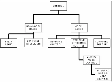
1.6 Literature Review

The purpose of manipulator control is to maintain the dynamic response of a manipulator in accordance with pre-specified objectives. The dynamic performance of a manipulator directly depends on the efficiency of the control algorithms and the dynamic model of the manipulator. Most of current industrial approaches to the robot arm control design treat each joint of the manipulator as a simple linear servomechanism with simple controller like Independent Joint Control (IJC), proportional plus derivative (PD), or proportional plus integral plus derivative (PID) controllers. In this approach, the nonlinear, coupled and time-varying dynamics of the mechanical part of the robot manipulator system have usually been completely ignored, or assumed as disturbances. However, when the links are moving

simultaneously and at high speed, the nonlinear coupling effects and the interaction forces between the manipulator links may decrease the performance of the overall system and increase the tracking error. The disturbances and uncertainties such as variable payload in a task cycle may also reduce the tracking quality of the robot manipulator system [Osman, 1991].

research area. Various advanced and sophisticated control strategies have been proposed by numerous researchers for controlling the robot manipulator such that the system is stable as well as the motion of the manipulator arm is maintained along the prescribed trajectory. The structures of these controllers can be grouped into three categories, the centralized, decentralized, and multilevel hierarchical structures. Many strategies have been developed for the centralized control schemes for improving the control of the nonlinear and coupled time varying robot manipulator. These include among others, the Computed Torque techniques [Craig, 1989], Adaptive control strategies [Ortega and Spong, 1988] and the Variable Structure Control approaches [Young, 1978].

Variable Structure Control (VSC) with sliding mode control was first proposed and elaborated in the early 1950’s in the Soviet Union by Emelyanov and several co-researchers. Since 1980, two developments have greatly enhanced the attention given to VSC systems. The first is the existence of a general VSC design method for complex systems. The second is a full recognition of the property of perfect robustness of a VSC system with respect to system perturbation and disturbances [John and James,1993].

A sliding mode will exist for a system if in the vicinity of the switching surface, the state vector is directed towards the surface. Filippov’s method is one possible technique for determining the system motion in a sliding mode, but a more straight forward technique easily applicable to multi-input systems is the method of equivalent control, as proposed by Utkin and Drazenovic [DeCarlo,et. al 1988].

known bounds. Such control strategies are based on the second method of Lyapunov. One have to take notice that, the plant uncertainties are required to lie in the image of input matrix B for all values of t and x. This requirement is the so-called matching condition [Gao and Hung, 1993]. The physical meaning of matching condition is that all modeling uncertainties and disturbances enter the system through the control channel [John and James,1993].

Sliding mode techniques are one approach to solving control problems and are an area of increasing interest. In the formulation of any control problem there will typically be discrepancies between the actual plant and the mathematical model developed for controller design. This mismatch may be due to any number of factors and it is the engineer's role to ensure the required performance levels exist despite the existence of plant/model mismatches. This has led to the development of so-called robust control methods. However this approach is decreasing the order of the system dynamics, may produce undesirable result in certain application. Other alternative must be introduce to increase the order of the closed-loop dynamics [Ahmad, 2003].

To overcome the problem of reduced order dynamics, a variety of the sliding mode control known as the Integral Sliding Mode Control has been successfully applied in a variety of control. Different from the conventional SMC design approaches, the order of the motion equation in ISMC is equal to the order of the original system, rather than reduced by the number of dimension of the control input. The method does not require the transformation of the original plant into the

1.7 Layout of Thesis

This thesis contained five chapters. Chapter 2 deals with the mathematical modelling of the direct drive robot arm. The formulation of the integrated dynamic model of this robot arm is presented. First, the state space representations of the actuator dynamics comprising of BLDCM motors are formulated. Then, the state space representations of the dynamic model of the mechanical linkage of the direct drive robot arm are established. Based on the actuator dynamics model, an

integrated dynamic model of the robot arm is presented.

Chapter 3 presents the controller design using integral sliding mode control. The direct drive robot arm is treated as an uncertain system. Based on the allowable range of the position and velocity of the direct drive robot arms operation, the model comprising the nominal and bounded uncertain parts is computed. Then, a

centralized control strategy for direct drive robot arm based on Integral Sliding Mode Control is described.

Chapter 4 discusses the simulation results. The performance of the Integral sliding mode controller is evaluated by simulation study using Matlab/Simulink. For the comparison purposes, the simulation study of Independent Joint Linear Control is also presented.

CHAPTER 2

MATHEMATICAL MODELING

2.1 Introduction

The most important initial step in the controlling an industrial robot is to obtain a complete and accurate mathematical model of the robot manipulator. This model is useful for computer simulation of the robot arm motion and synthesis processes before applied into real robot action.

The purpose of manipulator control is to maintain the dynamic response of a manipulator in accordance with pre-specified objectives. The dynamic performance of a manipulator directly depends on the efficiency of the control algorithms and the dynamic model of the manipulator [Ahmad, 2003]. Since the actuators are part of robot manipulator system, it is necessary to consider the effect of actuator dynamics. Therefore, it is important to include the actuators dynamic into the robot arm

dynamic equations.

The formulation of an integrated mathematical dynamic model of an

2DOF whose rigid links are jointed with revolute joints as shown in Figure 2.1 is considered. Both links of robot arm are actuated by brushless direct drive servo actuator BLDCM to drive the joints without gear reduction.

Figure 2.1 : 2 DOF Direct Drive Robot Arm [Reyes & Kelly,2001]

2.2 Brushless DC Motor (BLDCM) Dynamics

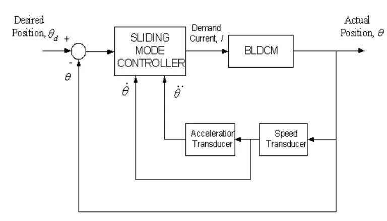
Figure 2.2 : Block Diagram of The Position Control of Each Joint of Robot

In order to proceed with the formulation of the integrated dynamic model of the direct drive robot manipulator, a complete set of dynamic equations of the actuators must be formulated first. The block diagram for the BLDCM as shown in Figure 2.2 is considered.

si si

si

R sL

R

+ sJi+Fi

1

s 1

i

K

L

T

θ& θ i

I

[image:30.612.135.519.70.289.2]

From the block diagram of the actuator, the equations of motion for the BLDCM can be obtained as follows [Karunadasa and Renfrew, 1991]:

) ( 1 ) ( ) ( ) ( ) ( )

( * T t

J t T L J R t I L J R K t L J R F t L R J F t _L i L si i si i si i si i i si i si i i si si i i

i && &

& _{− + − −}

⎟⎟⎠ ⎞ ⎜⎜⎝ ⎛ + − = θ θ

θ (2.1)

where

θ

&

_{: motor position (rad)}

θ

&&

_{: motor velocity (rad/s)}

θ

&

&

&

_{: motor acceleration (rad/s}2 )

i S

R

: motor stator winding resistance (Ω)

i S

L

: motor stator winding inductance (H)

t

K

: motor torque constant (N.m/A)

i

J

: motor rotor inertia (kg.m2)

i

F

: motor damping constant (kg.m2/s)

i

I

* : motor demand current (A)

i L

T

: motor load torque (N.m)

Define a 2x1 state vector of the ith actuator as

T i i

i

i t t t t

X ()=[θ () θ& ( ) θ&&()] (2.2)

Then equation (2.1) can then be written in state variable form as ) ( ) ( ) ( ) ( )

(t A X t B U t QT t W T t

X&_i = _{aci i} + _{aci i} + _{i Li} + _i &_Li (2.3)

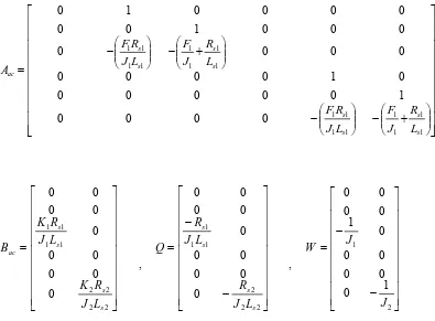
⎥ ⎥ ⎥ ⎦ ⎤ ⎢ ⎢ ⎢ ⎣ ⎡ = ⎥ ⎥ ⎥ ⎦ ⎤ ⎢ ⎢ ⎢ ⎣ ⎡ ⎟⎟⎠ ⎞ ⎜⎜⎝ ⎛ + − − = si i si i i ac si si i i si i si i i ac L J R K B L R J F L J R F A 0 , 0 1 0 0 ⎥ ⎥ ⎥ ⎦ ⎤ ⎢ ⎢ ⎢ ⎣ ⎡ − = si i si i L J R Q 0 ’ ⎥ ⎥ ⎥ ⎦ ⎤ ⎢ ⎢ ⎢ ⎣ ⎡ − = i i J W 1 0 ’ () *() t I t

U_i = _i (2.4)

with Xi(t) is a 2 x 1 state vector and Ui(t) is a scalar input of the ith actuator, while TLi(t) is the load acting on the ithactuator due to the manipulator links.

For a 2 DOF direct drive robot manipulator, the augmented dynamic equation of the actuators can be written in compact form as follows:

) ( ) ( ) ( ) ( )

(t A X t B U t QT t WT t

X& = _ac + _ac + _L + &_L (2.5)

where, T T T t X t X t

X()=[ ₁() ₂()]

T

t

U

t

U

t

U

(

)

=

[

₁

(

)

₂

(

)]

T L L

L t T t T t

T ( )=[ 1( ) 2()]

T L L

L t T t T t

T&()=[&₁() &₂()]

⎥ ⎥ ⎥ ⎥ ⎥ ⎥ ⎥ ⎥ ⎥ ⎥ ⎦ ⎤ ⎢ ⎢ ⎢ ⎢ ⎢ ⎢ ⎢ ⎢ ⎢ ⎢ ⎣ ⎡ ⎟⎟⎠ ⎞ ⎜⎜⎝ ⎛ + − ⎟⎟⎠ ⎞ ⎜⎜⎝ ⎛ − ⎟⎟⎠ ⎞ ⎜⎜⎝ ⎛ + − ⎟⎟⎠ ⎞ ⎜⎜⎝ ⎛ − = 1 1 1 1 1 1 1 1 1 1 1 1 1 1 1 1 0 0 0 0 1 0 0 0 0 0 0 1 0 0 0 0 0 0 0 0 0 0 0 1 0 0 0 0 0 0 1 0 s s s s s s s s ac L R J F L J R F L R J F L J R F A ⎥ ⎥ ⎥ ⎥ ⎥ ⎥ ⎥ ⎥ ⎥ ⎦ ⎤ ⎢ ⎢ ⎢ ⎢ ⎢ ⎢ ⎢ ⎢ ⎢ ⎣ ⎡ = 2 2 2 2 1 1 1 1 0 0 0 0 0 0 0 0 0 0 s s s s ac L J R K L J R K B , ⎥ ⎥ ⎥ ⎥ ⎥ ⎥ ⎥ ⎥ ⎥ ⎦ ⎤ ⎢ ⎢ ⎢ ⎢ ⎢ ⎢ ⎢ ⎢ ⎢ ⎣ ⎡ − − = 2 2 2 1 1 1 0 0 0 0 0 0 0 0 0 0 s s s s L J R L J R Q , ⎥ ⎥ ⎥ ⎥ ⎥ ⎥ ⎥ ⎥ ⎥ ⎦ ⎤ ⎢ ⎢ ⎢ ⎢ ⎢ ⎢ ⎢ ⎢ ⎢ ⎣ ⎡ − − = 2 1 1 0 0 0 0 0 0 1 0 0 0 0 J J W

[image:33.612.134.529.66.357.2]

The parameters of the Brushless DC Motor is as listed in Table 2.1 [Osman,1991]. Table 2.1: Parameters of the Actuators for Robot Arm

Notation Joint(Actuator) Parameter

1 2

Moment of Inertia Ji 2.85kg.m2 1.4kg.m2

Stator winding resistance Rsi 1.2Ω 1.3Ω

Stator winding inductance Lsi 0.162H 0.166H

Motor damping constant Fi 0.0573kg.m2/s 0.0253kg.m2/s

2.3 Modeling of Robot Dynamics

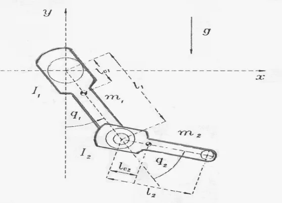
[image:34.612.209.488.126.327.2]

The configuration of the direct drive robot arm considered is as shown in Figure 2.4.

Figure 2.4 : The Configuration of 2 DOF Direct Drive Robot Arm [Reyes&Kelly, 2001]

The meaning and value of the physical of parameters of this robot arm [Reyes & Kelly, 2001] is as listed in Table 2.2:

Table 2.2 : List of Parameters of Robot Arm

Parameter Notation Value

Length link 1 l1 0.45m

Length link 2 l2 0.45m

Mass link 1 m1 23.902kg

Mass link 2 m2 1.285kg

Link (1) centre of mass lc1 0.091m

Link (2) centre of mass lc2 0.048m

Inertia link 1 I1 1.266kgm2

Inertia link 2 I2 0.093kgm2

[image:34.612.164.490.468.674.2]

The dynamics of a serial 2-link rigid robot shown in Figure 2.4 as follows [Reyes & Kelly,(2001)] : L T q f q g q q q C q q

M( )&&+ ( ,&)&+ ( )+ (&)= (2.4)

where;

q= joint displacements,

q&= joint velocities,

L

T =applied torque inputs,

M(q) = manipulator inertia matrix,

C(q, q&) =matrix of centripetal and Coriolis torques, g(q)= gravitational torques,

f(q&)=friction torques

Using the robot parameters as tabulated in Table 2.2, the entries for manipulator inertia, centripetal and Coriolis as well as gravitational torque is as follows [Reyes & Kelly,(2001)] : ⎥ ⎦ ⎤ ⎢ ⎣ ⎡ + + + = 102 . 0 ) cos( 084 . 0 102 . 0 ) cos( 084 . 0 102 . 0 ) cos( 168 . 0 351 . 2 ) ( 2 2 2 q q q q M ⎥ ⎦ ⎤ ⎢ ⎣ ⎡− − = 0 ) sin( 084 . 0 ) sin( 084 . 0 ) sin( 168 . 0 ) , ( 2 2 2 2 2 2 q q q q q q q q C & & & & ⎥ ⎦ ⎤ ⎢ ⎣ ⎡ + + + = ) sin( 186 . 0 ) sin( 186 . 0 ) sin( 921 . 3 ) ( 2 1 2 1 1 q q q q q q

g (2.5)

Define the system state variables as:

1

q&& = x₃ q&&₂ = x₆

1

q& = x2 q&2 = x5

1

q = x₁ q₂ = x₄ (2.6)

+ ⎥ ⎦ ⎤ ⎢ ⎣ ⎡ ⎥ ⎦ ⎤ ⎢ ⎣ ⎡ + + + = ⎥ ⎦ ⎤ ⎢ ⎣ ⎡ = 6 3 4 4 4 2 1 102 . 0 ) cos( 084 . 0 102 . 0 ) cos( 084 . 0 102 . 0 ) cos( 168 . 0 351 . 2 x x x x x

τ

τ

τ

⎥ ⎦ ⎤ ⎢ ⎣ ⎡ ⎥ ⎥ ⎥ ⎥ ⎦ ⎤ ⎢ ⎢ ⎢ ⎢ ⎣ ⎡ + − + + − 5 2 5 5 2 2 2 4 5 4 2 2 1 1 5 4 ) sgn( ) sin( 084 . 0 ) sin( 084 . 0 ) sgn( ) sin( 168 . 0 x x x x f b x x x x x x f b x x c c +

[ ]

1

1 4 1 1 4 1 1 ) sin( 8247 . 1 ) sin( 8247 . 1 ) sin( 465 . 38 x x x x x x x x ⎥ ⎥ ⎥ ⎥ ⎦ ⎤ ⎢ ⎢ ⎢ ⎢ ⎣ ⎡ + + + (2.7)

In the vector-matrix form, equation (2.7) can be represented as follows:

[ ]

1 21 11 5 2 22 21 12 11 6 3 22 21 12 11 2 1 x c c x x b b b b x x a a a a ⎥ ⎦ ⎤ ⎢ ⎣ ⎡ + ⎥ ⎦ ⎤ ⎢ ⎣ ⎡ ⎥ ⎦ ⎤ ⎢ ⎣ ⎡ + ⎥ ⎦ ⎤ ⎢ ⎣ ⎡ ⎥ ⎦ ⎤ ⎢ ⎣ ⎡ = ⎥ ⎦ ⎤ ⎢ ⎣ ⎡

τ

τ

(2.8)

Equation (2.8) can be rearranged into the following format:

⎥ ⎥ ⎥ ⎥ ⎥ ⎥ ⎥ ⎥ ⎦ ⎤ ⎢ ⎢ ⎢ ⎢ ⎢ ⎢ ⎢ ⎢ ⎣ ⎡ ⎥ ⎦ ⎤ ⎢ ⎣ ⎡ = ⎥ ⎦ ⎤ ⎢ ⎣ ⎡ = 6 5 4 3 2 1 22 22 21 21 21 12 12 11 12 11 2 1 0 0 x x x x x x a b a b c a b a b c T_L τ τ (2.9) or (2.10)

Differentiating equation (2.7) and rearranging it gives the derivative of applied torque inputs:

X x M

= ⎥ ⎦ ⎤ ⎢ ⎣ ⎡ = 2 1 τ τ & & & L

T _⎥+

⎦ ⎤ ⎢ ⎣ ⎡ ⎥ ⎦ ⎤ ⎢ ⎣ ⎡ + + + 6 3 4 4 4 102 . 0 ) cos( 084 . 0 102 . 0 ) cos( 084 . 0 102 . 0 ) cos( 168 . 0 351 . 2 x x x x x & & + ⎥ ⎦ ⎤ ⎢ ⎣ ⎡ ⎥ ⎦ ⎤ ⎢ ⎣ ⎡ − − − − − 6 3 2 2 4 2 4 4 5 4 4 1 ) sin( 084 . 0 ) sin( 168 . 0 ) sin( 084 . 0 ) sin( 168 . 0 ) sin( 168 . 0 x x b x x x x x x x x b _⎥+ ⎦ ⎤ ⎢ ⎣ ⎡ ⎥ ⎦ ⎤ ⎢ ⎣ ⎡ + − − 5 2 2 4 4 5 4 5 4 0 ) cos( 084 . 0 ) sin( 168 . 0 ) cos( 084 . 0 ) cos( 168 . 0 x x x x x x x x x (2.11)

[ ]

₁

1 4 1 4 1 1 4 1 4 1 1 ) cos( ) cos( 6494 . 3 ) sin( ) sin( 6494 . 3 ) cos( ) cos( 6494 . 3 ) sin( ) sin( 6494 . 3 ) cos( 465 . 38 x x x x x x x x x x x x ⎥ ⎥ ⎥ ⎥ ⎦ ⎤ ⎢ ⎢ ⎢ ⎢ ⎣ ⎡ + − + −

Equation (2.11) can be represented as follows:

[ ]

1 21 11 5 2 21 12 11 6 3 22 21 12 11 6 3 22 21 12 11 2 1

0 g x

g x x f f f x x e e e e x x d d d d

TL ⎥

⎦ ⎤ ⎢ ⎣ ⎡ + ⎥ ⎦ ⎤ ⎢ ⎣ ⎡ ⎥ ⎦ ⎤ ⎢ ⎣ ⎡ + ⎥ ⎦ ⎤ ⎢ ⎣ ⎡ ⎥ ⎦ ⎤ ⎢ ⎣ ⎡ + ⎥ ⎦ ⎤ ⎢ ⎣ ⎡ ⎥ ⎦ ⎤ ⎢ ⎣ ⎡ = ⎥ ⎦ ⎤ ⎢ ⎣ ⎡

⎥

⎥

⎥

⎥

⎥

⎥

⎥

⎥

⎦

⎤

⎢

⎢

⎢

⎢

⎢

⎢

⎢

⎢

⎣

⎡

⎥

⎦

⎤

⎢

⎣

⎡

6 5 4 3 2 1 22 22 22 21 12 12 11 12 11

0

0

0

x

x

x

x

x

x

e

e

f

g

e

f

e

f

g

(2.13)

In general equation (2.13) can be written as

(2.14)

Substituting equations (2.9) and (2.13) into the equation (2.5) gives

X&(t)= A_acX(t)+B_acU(t)+QM(x)X(t)+W[P(x)X&(t)+R(x)X(t)] (2.15)

Simplification of equation (2.15) provides the integrated dynamic model of the direct drive robot arm :

)) ( ) ( ) ( ) ( ) ( ) ( ( )] ( 1 [ )

(t WP x 1 A X t B U t QM x X t WR x X t

X& = − − _ac + _ac + + (2.16)

In general, equation (2.16) can be written as: ) ( ) ( ) ( ) ( )

(t A x X t B xU t

X& = + (2.17)

where

)}_A(_x) [1 _WP(_x)] 1{_{A QM}(_x) _WR(_x

ac + +

−

= − _(2.18)

} )] ( 1 {[ )

(x WP x 1Bac

B = − − (2.19)

X x R X x P

2.4 The Complete Integrated Model

The complete integrated model of a 2 DOF direct drive robot shown in Figure 2.1 can be obtained by substituting equation (2.10), (2.14), (2.18) and (2.19) into equation (2.17).

⎥⎦

⎤

⎢⎣

⎡

⎥

⎥

⎥

⎥

⎥

⎥

⎥

⎥

⎦

⎤

⎢

⎢

⎢

⎢

⎢

⎢

⎢

⎢

⎣

⎡

+

⎥

⎥

⎥

⎥

⎥

⎥

⎥

⎥

⎦

⎤

⎢

⎢

⎢

⎢

⎢

⎢

⎢

⎢

⎣

⎡

⎥

⎥

⎥

⎥

⎥

⎥

⎥

⎥

⎦

⎤

⎢

⎢

⎢

⎢

⎢

⎢

⎢

⎢

⎣

⎡

=

)

(

)

(

0

0

0

0

0

0

0

0

)

(

)

(

)

(

)

(

)

(

)

(

0

1

0

0

0

0

0

0

1

0

0

0

0

0

0

0

0

1

0

0

0

0

0

0

1

0

)

(

2 1 62 61 32 31 6 5 4 3 2 1 66 65 63 62 61 36 35 33 32 31

t

U

t

U

b

b

b

b

t

x

t

x

t

x

t

x

t

x

t

x

a

a

a

a

a

a

a

a

a

a

t

X

&

_(2.20)

Therefore, ) ( ) ( ) ( ) ( ) ( ) ( ) ( ) ( ) ( ) ( ) ( ) ( ) ( ) ( ) ( ) ( ) ( ) ( ) ( ) ( ) ( ) ( ) ( ) ( 2 62 1 61 6 66 5 65 3 63 2 62 1 61 6 6 5 5 4 2 32 1 31 6 36 5 35 3 33 2 32 1 31 3 3 2 2 1 t u b t u b t x a t x a t x a t x a t x a t x t x t x t x t x t u b t u b t x a t x a t x a t x a t x a t x t x t x t x t x + + + + + + = = = + + + + + + = = = & & & & & & where,

a31 =1.07/((-0.03-0.02cos(x4))(0.1+0.08cos(x4))+1.96+0.06cos(x4)) (0.07(38.47sin(x1)+1.82sin(x1+x4))/x1-0.35(38.47cos(x1)-

3.65sin(x1)sin(x4)+3.65cos(x1)cos(x4))/x1)+(-0.04-0.03cos(x4))/ ((-0.03-0.02cos(x4))(0.1+0.08cos(x4))+1.96+0.06cos(x4))(-0.28sin(x1+x4)/x1

-0.71(-3.65sin(x1)sin(x4)+3.65cos(x1)cos(x4))/x1)

(-0.16+0.01sin(x4)x5-0.49/x2+0.06cos(x4)x5)+(-0.04-0.03cos(x4))/ ((-0.03-0.02cos(x4))(0.1+0.08cos(x4))+1.96+0.06cos(x4))

(-.007sin(x4)x2-0.12sin(x4))

a33 =1.07/((-0.03-0.02cos(x4))(0.1+0.08cos(x4))+1.96+0.06cos(x4)) (-8.39-0.01cos(x4)+0.06sin(x4)+0.06sin(x4)x5)+(-0.04-0.03cos(x4))/ ((-0.03-0.02cos(x4))(0.1+0.08cos(x4))+1.96+0.06cos(x4))

(-0.02-0.01cos(x4)+0.06sin(x4)x2)

a35 =1.07/((-0.03-0.02cos(x4))(0.1+0.08cos(x4))+1.96+0.06cos(x4))(0.01sin(x4)x5 +0.03cos(x4)x5)+(-0.04-0.03cos(x4))/((-0.03-0.02cos(x4))(0.1+0.08cos(x4)) +1.96+0.06cos(x4))(-0.03-0.27/x5)

a36 =1.07/((-0.03-0.02cos(x4))(0.1+0.08cos(x4))+1.96+0.06cos(x4))

(-0.01-0.01cos(x4)+0.03sin(x4)+0.06sin(x4)x2)-7.99(-0.04-0.03cos(x4))/ ((-0.03-0.02cos(x4))(0.1+0.08cos(x4))+1.96+0.06cos(x4))

b31 = 1.07/((-0.03-0.02cos(x4))(0.1+0.08cos(x4))+1.96+0.06cos(x4))

b32 = (-0.04-0.03cos(x4))/((-0.03-0.02cos(x4))(0.1+0.08cos(x4)) +1.96+0.06cos(x4))

a61 = (-0.07-0.06cos(x4))/((-0.03-0.02cos(x4))(0.1+0.08cos(x4))+1.96+0.06cos(x4)) (-0.07(38.47sin(x1)+1.82sin(x1+x4))/x1-0.35(38.47cos(x1)-

3.65sin(x1)sin(x4)+3.65cos(x1)cos(x4))/x1)-(-1.82-0.06cos(x4 ))/((-0.03-2/95cos(x4))(0.1+0.08cos(x4))+1.96+0.06cos(x4))(-0.28sin(x1+x4)/x1 -0.71(-3.65sin(x1)sin(x4)+3.65cos(x1)cos(x4))/x1)

a62 = (-0.07-0.06cos(x4))/((-0.03-0.02cos(x4))(0.1+0.08cos(x4))+1.96+0.06cos(x4))

a63 =(-0.07-0.06cos(x4))/((-0.03-0.02cos(x4))(0.1+0.08cos(x4))+1.96+0.06cos(x4)) (-8.39-0.01cos(x4)+0.06sin(x4)+0.06sin(x4)x5)-(-1.82-28/475cos(x4))/

((-0.03-0.02cos(x4))(0.1+0.08cos(x4))+1.96+0.06cos(x4)) (-0.02-0.01cos(x4)+0.06sin(x4)x2)

a65 =(-0.07-0.06cos(x4))/((-0.03-0.02cos(x4))(0.1+0.08cos(x4))+1.96+0.06cos(x4)) (1701/296875sin(x4)x5+14/475cos(x4)x5)-(-1.82-28/475cos(x4))/

((-0.03-0.02cos(x4))(0.1+0.08cos(x4))+1.96+0.06cos(x4))(-0.03-0.27/x5)

a66 =(-0.07-0.06cos(x4))/((-0.03-0.02cos(x4))(0.1+0.08cos(x4))+1.96+0.06cos(x4)) (-0.01-0.01cos(x4)+0.03sin(x4)+0.06sin(x4)x2)+0.14(-1.82-28/475cos(x4))/ ((-0.03-0.02cos(x4))(0.1+0.08cos(x4))+1.96+0.06cos(x4))

b61 = (-0.07-0.06cos(x4))/((-0.03-0.02cos(x4))(0.1+0.08cos(x4))+1.96+0.06cos(x4))

CHAPTER 3

INTEGRAL SLIDING MODE CONTROL DESIGN

3.1 Overview of Controller

[image:43.612.133.521.63.349.2]

Figure 3.1 : Overview of Control Structure

3.2 Introduction to Variable Structure Control with Sliding Mode Control

In sliding mode control, the VSCS is designed to drive and then constrain the system state to lie within a neighborhood of the switching function. Its two main advantages are

a. the dynamic behavior of the system may be tailored by the particular choice of switching function.

b. the closed-loop response becomes totally insensitive to a particular class of

uncertainty. Also, the ability to specify performance directly makes sliding mode control attractive from the design perspective.

The idea of the sliding mode is simple: design a control law with varying control structures, and then force the trajectory of the system state to a certain

predefined surface, known as sliding surface, through an appropriate switching of the control structures such that the system dynamics are only determined by the

dynamics of the sliding surface.

3.3 Decomposition Into An Uncertain Systems

In order to apply the tracking controller based on the sliding mode control to the direct drive robot arm, the complete integrated dynamics of 2 DOF Direct drive robot given by equation (2.15) need to be decomposed into an uncertain dynamical system as shown below:

) ( )] , ( [ ) ( )] , ( [ )

(t A A xt X t B B xt U t

X& = +∆ + +∆ (3.1)

where T T T t X t X t

X()=[ ₁() ₂()]

[

]

T

t t t t

X( )= θ₁( ) θ&₁( ) θ&&()

T

t

U

t

U

t

U

(

)

=

[

₁

(

)

₂

(

)]

A and B are the nominal value of A and B respectively, with

2 MIN MAX A A

A= + (3.2)

and

2 MIN MAX B B

B = + (3.3)

On the other hand, ∆A and ∆B are uncertainty value of A and B respectively, with

MIN A A

A= −

∆ (3.4)

and ∆B=B−B_MIN (3.5)

The range of x₁,x₂,x₄ and x₅ as below

63 . 7 0 61 . 2 0 23 . 3 0 96 . 0 0 5 2 4 1 ≤ ≤ ≤ ≤ ≤ ≤ ≤ ≤ x x x x (3.6)

The nominal matrices A and B as well as the bounds on nonzero element of the matrices can be computed from the maximum and minimum value obtained from equation 3.2, 3.3, 3.4 and 3.5 an the results are tabulated in Table 3.1.

Table 3.1 : Value of Elements in Matrices A(x,t) and B(x,t)

MAX MIN NOMINAL ∆

a31 -5.1178 -15.8019 -10.45985 5.34205

a32 -0.8445 -2.4706 -1.65755 0.81305

a33 -4.3304 -4.7699 -4.55015 0.21975

a35 0.122 -0.1288 -0.0034 0.1254

a36 0.2524 0.0242 0.1383 0.1141

b31 0.5662 0.5331 0.54965 0.01655

b32 -0.0034 -0.0324 -0.0179 0.0145

a61 4.7334 -2.7852 0.9741 3.7593

a62 0.258 -0.0589 0.09955 0.15845

a63 0.5279 0.0547 0.2913 0.2366

a65 -0.0599 -0.1019 -0.0809 0.021

a66 -0.1345 -0.1363 -0.1354 0.0009

b61 -0.0069 -0.066 -0.03645 0.02955

Substituting the nominal values into equation (2.16) gives the system and input nominal matrices. ⎥ ⎥ ⎥ ⎥ ⎥ ⎥ ⎥ ⎥ ⎦ ⎤ ⎢ ⎢ ⎢ ⎢ ⎢ ⎢ ⎢ ⎢ ⎣ ⎡ − − − − − − = 1354 . 0 0809 . 0 0 2913 . 0 0996 . 0 9741 . 0 1 0 0 0 0 0 0 1 0 0 0 0 1383 . 0 0034 . 0 0 5502 . 4 6576 . 1 4599 . 10 0 0 0 1 0 0 0 0 0 0 1 0

A (3.7)

⎥ ⎥ ⎥ ⎥ ⎥ ⎥ ⎥ ⎥ ⎦ ⎤ ⎢ ⎢ ⎢ ⎢ ⎢ ⎢ ⎢ ⎢ ⎣ ⎡ − − = 9341 . 0 0365 . 0 0 0 0 0 0179 . 0 5497 . 0 0 0 0 0

B (3.8)

The uncertainties for system and input matrices can be obtained by substituting uncertainty value into equation (2.16)

⎥ ⎥ ⎥ ⎥ ⎥ ⎥ ⎥ ⎥ ⎦ ⎤ ⎢ ⎢ ⎢ ⎢ ⎢ ⎢ ⎢ ⎢ ⎣ ⎡ = ∆ 0009 . 0 021 . 0 0 2366 . 0 15845 . 0 7593 . 3 1 0 0 0 0 0 0 1 0 0 0 0 1141 . 0 1254 . 0 0 21975 . 0 81305 . 0 34205 . 5 0 0 0 1 0 0 0 0 0 0 1 0

⎥ ⎥ ⎥ ⎥ ⎥ ⎥ ⎥ ⎥

⎦ ⎤

⎢ ⎢ ⎢ ⎢ ⎢ ⎢ ⎢ ⎢

⎣ ⎡

= ∆

002 . 0 02955 . 0

0 0

0 0

0145 . 0 01655 . 0

0 0

0 0

B (3.10)

3.4 Problem Formulation

Consider the dynamics of the direct drive robot arm as an uncertain system described by equation (3.1).

Define the state vector of the system as

[

]

T

n t x t x t x t

X( )= ₁( ), ₂( ),..., ( ) (3.11)

Let a continuous function n d t R

X ()∈ be the desired state trajectory, where Xd(t) is

defined as:

[

]

T

dn d

d

d t x t x t x t

X ()= 1( ), 2(),..., ( ) (3.12)

Define the tracking error, Z(t) as

) ( ) ( )

(t X t X t

Z = − d (3.13)

In this study, the following assumptions are made:

i) The state vector X(t) can be fully observed;

ii) There exist continuous functions H(t) and E(t) such that for all n

R t

α

)

(

;

)

(

)

(

=

≤

∆

A

t

BH

t

H

t

(3.14(a))

) ( ;

) ( )

( = ≤

∆B t BE t E t (3.14(b))

iii) There exist a Lebesgue function Ω(t)∈R, which is integrable on bounded interval

such that

)

(

)

(

)

(

t

AX

t

B

t

X

d

=

_d

+

Ω

•

(3.15)

iv) The pair (A, B) is controllable.

In view of equations (3.13), (3.14) and (3.15), equation (3.10) can be written as an error dynamic system:

) ( )] ( [

) ( ) ( ) ( ) ( )] ( [

)

(t A BH t Z t BH t X t B t B BE t u t

Z• = + + _d − Ω + + (3.16)

Define the Proportional-Integral (PI) sliding surface as

∫

+

−

=CZ t t CA CBK Z d

t

0

) ( ] [

) ( )

( (3.17)

where C∈Rm×n and K∈Rm×n are constant matrices. The structure of the matrix C is as follows:

[ _{1 2} ]

i n c c c diag

C = L (3.18)

where n_ithe is the nth state variable associated to the ith input of the system. The matrix

C is chosen such that CB∈Rm×m is nonsingular.

The matrix K is designed to satisfy

0 ) (

The control problem is to design a controller using the PI sliding mode given by equation (3.17) such that the system state trajectory X(t) tracks the desired state trajectory Xd(t) as closely as possible for all t in spite of the uncertainties and

non-linearities present in the system.

3.5 System Dynamics During Sliding Mode

Differentiating equation (3.17) gives:

) ( ] [ ) ( )

(t = CZ• t − CA +CBK Z t

σ& (3.20)

Substituting equation (3.16) into equation (3.19) gives:

) ( ) ( )] ( [ ) ( ) ( ) ( ) ( ) ( )

(t =CBH t Z t +CBHt X_d t −CBΩt + CB+CBEt u t −CBKZt

σ& (3.21)

Equating equation (3.21) to zero gives the equivalent control, Ueq(t):

)} ( ) ( ) ( ) ( ) ( ) ( { )] ( [ )

(t CB CBEt 1 CBKZt CB t CBH t Z t CBHt X t

U_eq = + − + Ω − − _d (3.22)

Noting that 1 1 1 1 ) ( )] ( [ ))] ( )( [( )] (

[CB+CBEt − = CB In+Et − = In+Et − CB− (3.23)

the equivalent control of equation (3.22) can be written as

)} ( ) ( ) ( ) ( ) ) ( {( )] ( [ )

(t I E t 1 H t K Z t t H t X t

u_eq =− _n + − − −Ω + _d (3.24)

The system dynamics during sliding mode can be found by substituting the

equivalent control (3.24) into the system error dynamics (3.16). After simplification, it can be shown that:

Hence if the matching condition is satisfied (equation (3.14) holds), the system’s error dynamics during sliding mode is independent of the system uncertainties and couplings between the inputs, and, insensitive to the parameter variations.

3.6 Sliding Mode Tracking Controller Design

The manifold of equation (3.17) is asymptotically stable in the large, if the following hitting condition is held (Ahmad,2003):

0 ) ( ) ) ( / ) (

( T • <

t t

t

(3.26)

As a proof, let the positive definite function be )

( ) (t t

V =

(3.27)

Differentiating equation (3.26) with respect to time, t yields

) ( / )) ( ) ( ( ) ( T t t t t V i • • = (3.28)

Following the Lyapunov stability theory, if equation (3.26) holds, then the sliding manifold σ(t) is asymptotically stable in the large.

Theorem: The hitting condition (3.26) of the manifold given by equation (3.17) is satisfied if the control u(t) of system (3.16) is given by (Ahmad,2003):

) ( )) ( ( ] ) ( ) ( ) ( [ ) ( )

(t CB 1 ₁ Z t ₂ X t ₃ t SGN t t

u =− − + _d + Ω +Ω (3.29)

where ) 1 /( ) α (

1> CB + CBK + (3.30)

) 1 /( ) α (

2 > CB + (3.31)

) 1 /( ) (

Proof: Substituting equation (3.29) into equation (3.21) gives: ) ( ) ( ) ( ) ( )) ( ( } ) ( ) ( ) ( { ) )]( ( )[ ( ) ( ] ) ( [ ) ( 3 2 1 1 t t CBE t X t CBH t s SGN t t X t Z CB t E I CB t Z K t H CB t d d n Ω + + Ω + + + − − = −

σ

& (3.33)

Substituting equation (3.33) into (3.28) gives the rate of change of the Lyapunov function: ) ( ) ( ) ( )

(t V1 t V2 t V3 t

V • • • • + +

= (3.34)

where ))} ( ( ) ( ) )]( ( )[ ( ) ( ] ) ( [ { (t) ) ( ) ( 1 1

1 CBH t K Z t CB I E t CB Z t SGN t

t t V n T σ σ σ − • + − −

= (3.35)

))} ( ( ) ( ) )]( ( )[ ( ) ( ) ( { (t) ) ( )

( 1 ₂

2 CBH t X t CB I E t CB X t SGN t

t t

V _{d n d}

T σ σ σ − • + − = (3.36) ))} ( ( ) ( ) )]( ( )[ ( ) ( ) ( { (t) ) ( ) ( 3 1

3 CBE t t CB I E t CB t SGN t

t t V n T σ σ σ _{Ω − + Ω} = − • (3.37)

Now let simplify each Lyapunov term as follows. First term of equation (3.35):

) ( } α { ) ( } ) ( { (t) ) ( ) ( ]} ) ( [ { (t) ) ( t Z CBK CB t Z CBK t H CB t t Z K t H CB t T T + = + ≤ − σ_σ σ

σ _(3.38)

Noting that

(

)

1

) ( ) ( ) ( ) ( ) ( ) ( ) ( )) ( ( ) ( ) ( 2

2 = =

= t t t t t t t t SGN t t T T T T σ σ σ σ σ σ σ σ σ

σ _(3.39)

then the second term of (3.35) can be simplified as

Using equation (3.38) and (3.40), equation (3.35) can be written as

) ( ]}

[α

) {(1 )

( 1

1 t CB CBK Z t

V• ≤− + − + (3.41)

Similarly, equation (3.36) and (3.37) can be simplified in a same manner and the results are summarized as follows:

) ( }

α

) {(1 )

( 2

2 t CB X t

V ≤ − + − d

•

(3.42)

) ( } )

{(1 )

( ₃

3 t CB t

V ≤ − + − Ω

•

(3.43)

CHAPTER 4

SIMULATION RESULTS

4.1 Introduction

A complete set of non-linear dynamic equations of the robot model comprising the mechanical part of the robot and the actuator dynamics have been derived and used in the simulations. The equations are highly non-linear and coupled, taking into account the contributions of the actuator dynamics, as well as the inertias, the

4.2 Trajectory Generation

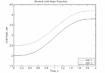
A trajectory is defined as a time history of position, velocity and acceleration of each joint of robot arm. The controller is required to track a pre-specified reference trajectory for the joint angle is generated by the cycloidal function, as follows (Osman, 1991):

⎪⎩ ⎪ ⎨ ⎧

≤ ≤ ≤ −

∆ + =

t t t

t t

i i i

di

τ τ

θ

τ τπ

τπ π θ

θ

), (

0 )], 2 sin( 2

[ 2 ) 0 ( )

( (4.1)

where,

. 2 2

, 1 ), 0 (

θ

) (

θi i i s

i = − = =

[image:55.612.155.378.224.307.2]

∆ τ

Figure 4.1 below shows the desired joint angle trajectories for both joints.

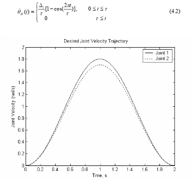
[image:55.612.141.509.338.596.2]

By differentiating equation (4.1) with respect to time, t gives the smooth bell shaped velocity profile as shown in the figure 4.2.

⎪⎩ ⎪ ⎨ ⎧

≤ ≤ ≤ −

∆ =

t t t

t i

di

τ τ τπ

τ θ

0

0 )], 2 cos( 1 [ )

(

[image:56.612.133.516.123.482.2]

& _(4.2)

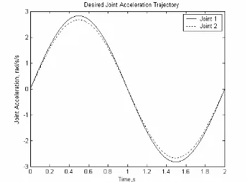
The acceleration profile can be generated by differentiating equation (4.2) with respect to time, t. The sinusoidal acceleration profile as follows:

⎪⎩ ⎪ ⎨ ⎧

≤ ≤ ≤ ∆

=

t t t

t

i

di

τ τ τπ

τπ θ

0

0 )], 2 sin( 2

)

( 2

&

& _(4.3)

[image:57.612.151.502.219.477.2]

Figure 4.3 below shows the desired acceleration profile for both joints of direct drive robot arm.

Figure 4.3 : Desired Joint Acceleration Profile For Both Joints

The joint trajectories for both joints are set to start at the initial position of T

T

] 5 . 1 8 . 0 [ ] ) 0 ( ) 0 (

[θ₁ θ₂ = − − radians, to a desired final position of T

T

t

t) ()] [1 0.2] (

4.3 Simulation Using Independent Joint Linear Control (IJC)

Independent Joint Linear Control method is normally used in most industrial robot. The simulation study is used as comparison to the Integral Sliding Mode Control. Through this simulation, the performance of the IJC can be evaluated when applied to the non linear, time varying and coupled dynamics of the direct drive robot arm.

This controller is designed with the dynamics of the mechanical linkage completely ignored. Each joint of the robot arm is treated as an independent servomechanism problem represented by an actuator state equation as follows:

) ( )

( )

(t A X t B U t

X _{ac i ac i}

i

i +

=

& _(4.4)

The element of matrices i ac A and

i ac

B are similar as described in equation 2.4. Based on the actuator parameters value tabulated in Table 2.1, the matrices

i ac A and i ac

B are calculated as follows:

⎥ ⎥ ⎥ ⎦ ⎤ ⎢ ⎢ ⎢ ⎣ ⎡ − − = 4275 . 7 0039 . 0 0 1 0 0 0 1 0 1 ac

A ;

⎥ ⎥ ⎥ ⎦ ⎤ ⎢ ⎢ ⎢ ⎣ ⎡ = 0081 . 2 0 0 1 ac B ⎥ ⎥ ⎥ ⎦ ⎤ ⎢ ⎢ ⎢ ⎣ ⎡ − − = 8494 . 7 0039 . 0 0 1 0 0 0 1 0 2 ac

A ;

⎥ ⎥ ⎥ ⎦ ⎤ ⎢ ⎢ ⎢ ⎣ ⎡ = 4343 . 3 0 0 2 ac

B (4.5)

The linear state feedback controller employed in each of the joint is described as follows: ) ( ) ( )

(t K Z t t

U_i = _{i i} +Ω_i (4.6)

i

K - 1x3 linear state feedback gain )

(t i

Ω - control component to eliminate the steady state error

) ( )

( )

(t X t X t

Zi = i − d_i (4.7)

Each of the sub-system has been assigned with the following closed-loop poles:

} 1 5 . 1 2 { ) (

λi Ai ₊BiKi _{= − − −} ; i=1,2 (4.8)

All desired poles are located in the left half plane to ensure stability.

Using the pole-placement method, the values of feedback gains are obtained as follows:-

Sub-system 1 : K₁ =

[

1.4939 3.2349 −1.4578

]

Sub-system 2 : K₂ =

[

0.8735 1.8915 −0.9753

]

(4.9)

[image:60.612.148.496.69.332.2] [image:60.612.134.498.82.639.2]

Figure 4.4 : Tracking Response of Joint 1 with IJC

4.4 Simulation Using Integrated Sliding Mode Controller

In this section the simulation is carried out using the controller described by equation (3..29).

4.4.1 The Selection of Controller Parameters

The three values that will determine the shape of the plant output in response to the desired input trajectory are (Ahmad,2003)

a. Sliding Surface Constant, C

The constant c , _n in equation (3.18) will determine the magnitude of the ith input,U_i(t), while the constants ₁, ₂, ₋₁

i n c c

c L will determine the shape of the trajectories during the reaching phase.

b. The Desired Poles Location

The desired poles location can be placed anywhere on the left half plane (LHP) of the s-plane to guarantee stability during the sliding phase. However, if the locations of the desired closed-loop poles are placed too far on the LHP of the s-plane, high gain K will be produced and will somehow affects the shape of the PI sliding surface of equation (3.17).

c. Integral Sliding Mode Controller Parameters,γ

Algorithm 4.1 :

Step 1. Input data: Numerical values for C =diag[c1, c2 ... cn_i],

max

λ (A + BK) < 0, and γ_i> o.

Step 2. Check if the sliding mode exists and whether the output tracking response is satisfactory. If the conditions do not hold then try other combinations. If the conditions hold, proceed to Step 3.

Step 3. Check if all of the control inputs T m t U t

U t U t

U()=[ ₁() ₂() .... ( )] are within the admissible range. If the condition does not hold then increase the value of c , _n and place the desired poles closer to the origin until sliding mode exist and the control input U(t) is within the admissible limit. If the condition holds, then proceed to Step 4.

Step 4. Check if the output trajectories are satisfactory during the reaching phase. If the conditions do not hold then adjust the values of c1, c2 ... c n_i until

satisfactory shape of the output trajectories are achieved. If the conditions hold, then proceed to Step 5.

Step 5. Check if the tracking errors of the output trajectories are satisfactory. If the conditions do not hold then increase the values of γ_i ,for i = 1,2,3 until satisfactory tracking errors are achieved. The values of γ_i should not be too large to guarantee that the control input U(t) is within the admissible limit. If the conditions hold, then go to Step 6.

Step 6. Finish.

4.4.2 Numerical Computation

As stated in Chapter 3, the pair (A, B) is controllable. Controllability deals with whether or not the state of a state space equation can be controlled from the input. The pair (A, B) is controllable if for any initial state x(0)= x₀ and any final state x₁, there exists on input that transfers x₀ tox₁ in a finite time. Otherwise (A, B) is said to be uncontrollable ( Chi Tsong, 1999). Controllability of the pair (A, B) can be tested by a controllability matrix

] [ 2 B A AB B

P∆= M M (4.10)

n- dimensional continuous time system is completely controllable if and only if the matrix has rank n.

By using equation (3.7) and (3.8), the rank of

⎥ ⎥ ⎥ ⎥ ⎥ ⎥ ⎥ ⎥ ⎦ ⎤ ⎢ ⎢ ⎢ ⎢ ⎢ ⎢ ⎢ ⎢ ⎣ ⎡ − − − − − − − − − − − − − = 0018 . 0 6947 . 0 1317 . 0 1651 . 0 9341 . 0 0365 . 0 1317 . 0 1651 . 0 9341 . 0 0365 . 0 0 0 9341 . 0 0365 . 0 0 0 0 0 9501 . 0 5159 . 10 2106 . 0 5063 . 2 0179 . 0 5497 . 0 2106 . 0 5063 . 2 00179 5497 . 0 0 0 0179 . 0 5497 . 0 0 0 0 0

P (4.11)

is 6, so that the pair (A, B) is controllable.

The bounds of H(t) may be computed as follows using equation (3.14(a))

) ( ] ) [( ) ( 1 t A B B B t

H = T − T ∆ (4.12)

where, (BTB)−1BT is called the pseudo inverse.

Hence, ⎥⎦ ⎤ ⎢⎣ ⎡ = 0091 . 0 0314 . 0 0 2692 . 0 2277 . 0 4099 . 4 2079 . 0 2291 . 0 0 4075 . 0 4865 . 1 8617 . 9

H (4.13)

Therefore,

9223 . 10 ≥

α

(4.14)

However, the bounds of E(t) may be computed as follows using equation (3.14(b)) ) ( ] ) [( )

(t B B 1B B t

E = T − T ∆

Hence, ⎥⎦ ⎤ ⎢⎣ ⎡ = 0.0032 0.0329 0.0265 0.0312 ) (t E

and β ≥ E(t) Therefore, 0267 . 0 ≥ β (4.11)

Define the gain K as:

⎥⎦ ⎤ ⎢⎣ ⎡− − = 6883 . 4 8805 . 6 2157 . 3 3087 . 0 4514 . 0 5132 . 0 4043 . 0 2179 . 0 1047 . 0 0813 . 0 8239 . 8 5541 . 13

K (4.12)

such that the closed-loop poles of the system are: Joint 1: λ1 ={−1,−1.5,−2)

Joint 2: λ2 ={−1,−1.5,−2) (4.13)

The desired poles location can be placed anywhere on the left half plane (LHP) of the s-plane to guarantee stability during the sliding phase

Define the matrix C as:

⎥⎦ ⎤ ⎢⎣ ⎡ = 1 20 30 0 0 0 0 0 0 1 3 2 ) (t

C (4.14)

Using (3.34), (3.35) and (3.36), the controller parameter γ may be computed as follows: 0243 . 0 ; 9582 . 9 ; 7959 .

18 _{2 3}

4.4.3 The Effect of the Value of Controller Parameter, γ

The effect of the controller parameter γ is studied in this section. For comparison purposes, two sets of the controller parameters are chosen as shown in Table 4.1:

Table 4.1: Two Sets of Controller Parameters Set 1

(Unsatisfied the condition)

Set 2

(Satisfied the condition)

1

γ

10 36

2

γ 5 20

3

γ 0.01 0.875

In Set 1, the controller parameters are selected to study the performance of the system if the controller parameters’ conditions of equations (3.34)-(3.36) are unfulfilled, while in Set 2 the controller parameters is selected to represent a situation where the conditions are fulfilled.

[image:67.612.152.503.68.326.2]

Figure 4.6 : Tracking Response of Joint 1 with Unsatisfied Controller Parameters

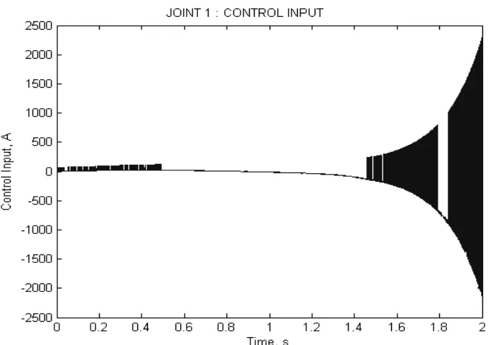
[image:67.612.155.502.399.664.2]

[image:68.612.143.488.68.312.2]

Figure 4.8 : Joint 1 Control Input of PISMC with Unsatisfied Controller Parameters

[image:68.612.141.494.407.651.2]

[image:69.612.137.497.67.293.2]

Figure 4.10 : Joint 1 Sliding Surface of PISMC with Unsatisfied Controller Parameters

[image:69.612.137.494.383.610.2]

[image:70.612.135.502.262.518.2]

However the actual output positions can track the desired trajectory if the controller parameter conditions are satisfied. The good tracking performance results for joint 1 as shown in the Figure 4.12 and for joint 2 as in Figure 4.13. From the result obtained the direct drive robot arm able to track the desired trajectory if the conditions of sliding mode controller parameters are fulfilled. The control input generated for joint 1 and joint 2 switches very fast as shown in Figure 4.14 and 4.15, respectively. . The sliding surfaces of joint 1 and joint 2 as shown in Figure 4.10 and 4.11, respectively.

[image:71.612.136.504.67.330.2]

Figure 4.13 : Tracking Response of Joint 2 with Satisfied Controller Parameters

[image:71.612.150.478.399.605.2]

[image:72.612.151.478.67.271.2]

Figure 4.15 : Joint 2 Control Input of PISMC with Satisfied Controller Parameters

[image:72.612.135.497.362.579.2]

[image:73.612.132.471.69.282.2]

4.6 Control Input Chattering Suppression

[image:74.612.208.482.268.484.2]

In the presence of switching imperfections, such as switching time delays and small time constants in the actuators, the discontinuity in the feedback control produces a particular dynamics behavior in the vicinity of the surface, which is commonly referred to as chattering (Perruquet