Small area estimation with time and area effects using a dynamic linear model

(1)

(2)

ix

Inventory Model With Gamma Distribution

Hadi Sumadibrata, Ismail

Bin Mohd

642

Accuracy Analysis Of Naive Bayesian

Anti-Spam Filter

Ruslam, Armin Lawi, And

Sri Astuti Thamrin

649

A New Method For Generating Fuzzy Rules From Training Data

And Its Application In Financial Problems

Agus Maman Abadi,

Subanar, Widodo, Samsubar

Saleh

655

The Application Of Laws Of Large Numbers In Convergence

Concept In Probability And Distribution

Georgina M. Tinungki

662

An Empirical Bayes Approach for Binary Response Data in

Small Area Estimation

Dian Handayani, Noor

Akma Ibrahim, Khairil A.

Notodiputro, MOhd. Bakri

Adam

669

Statistical Models For Small Area Estimation

Khairil A Notodiputro,

Anang Kurnia, and Kusman

Sadik

677

Maximum Likelihood Estimation For The Non-Separable Spatial

Unilateral Autoregressive Model

Norhashidah Awang,

Mahendran Shitan

685

Small Area Estimation Using Natural Exponential Families With

Quadratic Variance Function (Nef-Qvf) For Binary Data

Kismiantini

691

Using An Extended And Ensemble Kalman Filter Algorithm For

The Training Of Feedforward Neural Network In Time Series

Forecasting

Zaqiatud Darojah, M. Isa

Irawan, And Erna Apriliani

696

Estimation Of Outstanding Claims Liability And Sensitivity

Analysis: Probabilistic Trend Family (PTF) Model

Arif Herlambang, Dumaria

R Tampubolon

704

Expected Value Of Shot Noise Processes

Suyono

711

Modelling Malaysian Wind Speed Data Via Two Paramaters

Weibull

Nur Arina Basilah Kamisan,

Yong Zulina Zubairi, Abdul

Ghapor Hussin, Mohd.

Sahar Yahya

718

Application Of Latin Hypercube Sampling And Monte Carlo

Simulation Methods: Case Study The Reliability Of Stress

Intensity Factor And Energy Release Rate Of Indonesian

Hardwoods

Yosafat Aji Pranata And

Pricillia Sofyan Tanuwijaya

726

The Development Of Markov Chain Monte Carlo (Mcmc)

Algorithm For Autologistic Regression Parameters Estimation

Suci Astutik, Rahma

Fitriani, Umu Sa’adah, And

Agustin Iskandar

734

A Note About Dh-Fever Estimation With ARIMAX Models

Elly Ana, Dwi Atmono

Agus W

741

Evaluation Of Additive-Innovational Outlier Identification

Procedure For Some Bilinear Models

I

smail, M.I., Mohamed, I.B.,

Yahya, M.S.

(3)

xi

Model By Spectral Regression Methods

Iriawan, Suhartono

Application Of Cluster Analysis To Developing Core Collection

In Plant Genetic Resources

Sutoro

875

Small Area Estimation With Time And Area Effects Using A

Dynamic Linear Model

Kusman Sadik And Khairil

Anwar Notodiputro

880

Statistical Analysis Of Wind Direction Data

Ahmad Mahir Razali, Arfah

Ahmad, Azami Zaharim

And Kamaruzzaman Sopian

886

Generalized Additive Mixed Models in Small Area Estimation

Anang Kurnia, Khairil A.

Notodiputro, Asep

Saefuddin, I Wayan

Mangku

891

Kernel Principal Component Analysis In Data Visualization

Ismail Djakaria, Suryo

Guritno, Sri Haryatmi

898

GARCH Models And The Simulations

Nelson Nainggolan, Budi

Nurani Ruchjana And

Sutawanir Darwis

906

Rainfall Prediction Using Bayesian Network

Hera Faizal Rachmat, Aji

Hamim Wigena, and Erfiani

911

Identifying Item Bias Using The Simple Volume Indices And

Multidimensional Item Response Theory Likelihood Ratio

(Irt-Lr) Test

Heri Retnawati

916

Ordinary Kriging And Inverse Distance Weighting For Mapping

Soil Phosphorus In Paddy Field

Mohammad Masjkur,

Muhammad Nuraidi and

Chichi Noviant

924

K-Means Clustering Visualization

On Agriculture Potential Data

For Villages In Bogor Using Mapserver

Imas S. Sitanggang, Henri

Harianja, and Lailan

Syaufina

932

Some Methods To Estimate The Number Of Components In A

Mixture

M. A. Satyawan, A. H.

Wigena, Erfiani

941

A Probabilistic Model For Finding A Repeat

Triplet Region In DNA Sequence

Tigor Nauli

947

Application Of Spherical Harmonics In Determination Of Tec

Using Gps Observable

Mardina Abdullah, Siti

Aminah Bahari, Baharudin

Yatim, Azami Zaharim,

Ahmad Mahir Razali

954

Testing Structure Correlation Of Global Market By Statistic Vvsv Erna Tri Herdiani, and

Maman A. Djauhari

961

Exploring the MAUP from a spatial perspective

Gandhi Pawitan

967

Estimation of RCA(1) Model using EF:

A new procedure and its robustness

1Norli Anida Abdullah,

2Ibrahim Mohamed,

3Shelton Peiris

996

Second Order Linear Elliptic Operators

In The Unit Square

(4)

xii

POSTER

Study Of Fractional Factorial Split-Plot Experiment

Sri Winarni, Budi Susetyo,

and Bagus Sartono

1012

Improving Model Performance For Predicting Poverty Village

Category Using Neighborhood Information In Bogor

Bagus Sartono, Utami Dyah

S, and Zulhelmi Thaib

1019

Ammi Models On Count Data: Log-Bilinear Models

Alfian Futuhul Hadi

H. Ahmad Ansori Mattjik

I Made Sumertajaya

Halimatus Sa’diyah

1026

Prediction Of Oil Production Using Non Linear Regression By

Sdpro Software

(Special Program Package)

*)

Budi Nurani R , and

Kartlos J. Kachiashvili

1038

An Implementation Of Spatial Data Mining

Using Spatial Autoregressive (Sar) Model

For Education Quality Mapping At West Java

*)

Atje Setiawan A. ,

Retantyo Wardoyo , Sri

Hartati , and Agus Harjoko

1045

Validation Of Training Model

For Robust Tests Of Spread

Teh Sin Yin, and Abdul

Rahman Othman

1056

Spectral Approach For Time Series Analysis

Kusman Sadik

1063

The ACE Algorithm for Optimal Transformations in Multiple

Regression

Kusman Sadik

1066

The Relation Between The Students’ Interaction And The

Construction Of Mathematical Knowledge

Rini Setianingsih

1069

Application of Auto Logistic Regression Spatial Model using

Variogram Based Weighting Matrix to Predict Poverty Village

Introduction

The problem of small area estimation is how to produce reliable estimates of area (domain) characteristics, when the sample sizes within the areas are too small to warrant the use of traditional direct survey estimates. The term of small area usually denote a small geographical area, such as a county, a province, an administrative area or a census division. From a statistical point of view the small area is a small domain, that is a small sub-population constituted by specific demographic and socioeconomic group of people, within a larger geographical areas. Sample survey data provide effective reliable estimators of totals and means for large areas and domains. But it is recognized that the usual direct survey estimators performing statistics for a small area, have unacceptably large standard errors, due to the circumstance of small sample size in the area. In fact, sample sizes in small areas are reduced, due to the circumstance that the overall sample size in a survey is usually determined to provide specific accuracy at a macro area level of aggregation, that is national territories, regions ad so on (Datta and Lahiri, 2000).

Demand for reliable small area statistics has steadily increased in recent years which prompted considerable research on efficient small area estimation. Direct small area estimators from survey data fail to borrow strength from related small areas since they are based solely on the sample data associated with the corresponding areas. As a result, they are likely to yield unacceptably large standard errors unless the sample size for the small area is reasonably large(Rao, 2003). Small area efficient statistics provide, in addition of this, excellent statistics for local estimation of population, farms, and other characteristics of interest in post-censual years.

(6)

881

census and specific sample surveys records. Small area efficient statistics provide, in addition of this, excellent statistics for local estimation of population, farms, and other characteristics of interest in post-censual years.

2.

Direct estimation

Sample surveys have long been recognized as cost-effective means of obtaining information on wide-ranging topics of interest at frequent intervals over time. They are widely used in practice to provide estimates not only for the total population of interest but also for a variety of sub-populations (domains). Domain may be defined by geographic areas or socio-demographic groups or other sub-population. Examples of geographic domain (area) include a state/province, county, municipality, school district, unemployment insurance region, metropolitan area, and health service area. On other hand, a socio-demographic domain may refer to a specific age-sex-race group within a large geographic area. An example of other domains is the set of business firms belonging to a census division by industry group (Rao, 2003).

Direct estimation usually is based on under the design-based or repeated sampling framework. The technique have been developed by Sewnson dan Wretman (1992). Model-based methods have also been used to develop direct estimators and associated inferences. Such methods provide valid conditional inferences refering to the particular sample that has been drawn, regardless of the sampling design (see Pffermann, 2002).

A sampling design is used to select a sample s from U with probability p(s). The sample selection

probability p(s) can depend on know design variables such as stratum indicator variables and size

measures of clusters. Design weights wj(s) play an important role in constructing design-based estimator

Y

ˆ

of Y. These basic weights may depend both on s and the element j (j∈s). An important choice is

wj(s)=1/πj, where πj = Σ{s:j∈s}p(s), j=1, 2, .., N. In the absence of auxiliary population information, we use

expansion estimator

Y

ˆ

= Σ{s:j∈s}wj(s)yj. In this case, the design-unbiased condition reduces to

Σ{s:j∈s}p(s)wj(s) = 1, j=1, 2, …, N. The choice wj(s)=1/πj satisfies the unbiased condition and leads to the well-known Horvits-Thompson estimator.

Rao (2003) has shown that a non-negative unbiased quadratic estimator of variance of

Y

ˆ

is necessarily of

the form

2

,

) ( )

ˆ

(

∑ ∑

< ∈ 

   

  

− −

= k

j jk s k

k j j k j jk

b y b y b b s w Y

v

where the weights wjk(s) satisfy the unbiased condition and the non-zero constants bjand bk.

Direct estimation can also use auxiliary information. Suppose now that auxiliary information in the form of known population totals X = (X1, …, Xp)

T

is available and that the auxiliary vector xj for j∈s is also observed, that is, the data (yj, xj) for each element j∈s are observed. An estimator that makes efficient use of this auxiliary information is generalized regression (GREG) which may be written as:

B X X ˆ) ˆ (

ˆ

ˆ T

GR Y

Y = + −

where Xˆ= Σ{s:j∈s}wj(s)xj and Bˆ=(Bˆ₁,...,Bˆ_p)T is the solution of sample weighted least squares equations:

(Σ{s:j∈s}wj(s)xjxj T

/cj)

B

ˆ

= Σ{s:j∈s}wj(s)xjyj/cj

with specified constants cj(>0).

3.

Indirect estimation in small area

(7)

882

small sample size include local area, sub-domain, small subgroup, sub-province, and minor domain. In some applications, many domains of interest (such as counties) may have zero sample size.

Three types of indirect estimators can be identified : domain indirect, time indirect, and domain and time

indirect. A domain indirect estimator makes use of y-values from another domain but not from another

time period. A time indirect estimator uses y-values from another time period for the domain interest but

not from another domain. On the other hand, a domain and time indirect estimator uses y-values from

another domain as well as another time period (Rao, 2003).

In making estimates for small area with adequate level of precision, it is often necessary to use indirect

estimators that borrow strength by using thus values of the variable of interest, y, from related areas

and/or time periods and thus increase the effective sample size. These values are brought into the estimation process through a model (either implicit or explicit) that provides a link to related areas and/or

time periods through the use of supplementary information related to y, such as recent census counts and

current administrative records (Pfeffermann 2002; Rao 2003).

Methods of indirect estimation are based on explicit small area models that make specific allowance for

between area variation. In particular, we introduce mixed models involving random area specific effects

that account for between area variation beyond that explained by auxiliary variables included in the

model. We assume that θi = g(

Y

i) for some specified g(.) is related to area specific auxiliary data zi = (z1i, …, zpi)

T

through a linear model

θi = zi T_β

+ bivi, i = 1, …, m

where the bi are known positive constants and βis the px1 vector of regression coefficients. Further, the vi are area specific random effects assumed to be independent and identically distributed (iid) with

Em(vi) = 0 and Vm(vi) = σv 2

(≥ 0), or vi∼ iid (0, σv 2

)

4.

Time series and cross-sectional models

Many sample surveys are repeated in time with partial replacement of the sample elements. For such repeated surveys considerable gain in efficiency can be achieved by borrowing strength across both small areas and time. Rao and Yu (1992, 1994) proposed an extension of the basic Fay-Herriot model to handle time series and cross-sectional data. Their model consist of a sampling error model

=

θˆit θit + eit, t = 1, …, T; i = 1, …, m

and a linking model

θit = zit

T_β

+ vi + uit

Here

θ

ˆ

_it is the direct survey estimator for small area i at time t, θit is a function of the small area mean,

the eit are sampling error normally distributed with zeros means and a known block diagonal covariance

matrix ψ, and zit is a vector of area specific covariates some of which may change with t, for example,

administrative data. Further, vi∼ iid (0, σv 2

) and uit are assumed to follow a random walkprocess for each

i, that is,

uit = ui,t-1 + εit, dan εit∼iid N(0, σ 2

)

The errors {eit}, {vi}, and {εit} are also assumed to be independent. The model on θit depends on both area specific effects vi and the area-by-time specific effects uit which are correlated across time for each i.

5.

Generalized linear mixed model

Datta and Lahiri (2000), and Rao(2003) considered a general linear mixed model (GLMM) which covers the univariate unit level model as special cases:

yP = XPβ+ ZPv + eP

Hence v and eP are independent with eP∼N(0, σ2ψP) and v∼N(0, σ2D(λ)), where ψP is a known positive

(8)

883

parameters λ typically involving ratios of variance components of the form σi

2

/σ2. Further, XPand ZP are

known design matrices and yP is the N x 1 vector of population y-values. The GLMM form :

      +       +       =       = * e e v * Z Z * X X * y y

yP β

where the asterisk (*) denotes non-sampled units. The vector of small area totals (Yi) is of the form Ay +

Cy* with A = _im T_n

i

1

=

⊕

and C = m_i T_N _n

i i−

=

⊕

₁

1

where m _u

i=1A

⊕ = blockdiag(A1, …, Am).

We are interested in estimating a linear combination, µ = 1Tβ + mTv, of the regression parameters β and

the realization of v, for specified vectors, l and m, of constants. For known δ, the BLUP (best linear

unbiased prediction) estimator of µ is given by (Rao, 2003)

H

µ

~

_{= t(}_δ_,_y_{) =}₁T

β

~

+ mT

~

v

= 1T

β

~

+ mTGZTV-1(y - X

β

~

)

Model of indirect estimation,

θ

ˆ

i

=

ziTβ + bivi+ ei, i = 1, …, m, is a special case of GLMM with block diagonal covariance structure. Making the above substitutions in the general form for the BLUP estimator

of µi, we get the BLUP estimator of θi as:

H i

θ

~

= zi T

β

~

+ γi(

θ

ˆ

i - zi T

β

~

), where γi = σv 2

bi 2

/(ψi + σv 2

bi 2

), and

β

~

=

β

~

(σv2) =

        σ + ψ θ         σ + ψ

∑

= − = m

i i v i

i i m

i i v i

T i i b b 1 2 2 1 1 2 2 ˆ z z z

6.

Dynamic linear model

Many sample surveys are repeated in time with partial replacement of the sample elements. For such repeated surveys considerable gain in efficiency can be achieved by borrowing strength across both small areas and time. Their model consist of a sampling error model

=

θ

ˆ

it θit + eit, t = 1, …, T; i = 1, …, m

θit = zitTβit where the coefficients βit = (βit0, βit1, …, βitp)

T

are allowed to vary cross-sectionally and over time, and the sampling errors eit for each area i are assumed to be serially uncorrelated with mean 0 and variance ψit. The variation of βit over time is specified by the following model:

p j vitj ij j t i j ij itj ,..., 1 , 0 , 0 1 β β β

β _, ₁_,

=       +       =       − T

It is a special case of the general dynamic linear model (state-space model) which may be expressed in the form

yt = Ztαt + εt; E(εt) = 0, E(εtεt

T

) = Σt

αt = Htαt-1 + Aηt; E(ηt) = 0, E(ηtηtT) = Γ

where εt and ηt are uncorrelated contemporaneously and over time. The first equation is known as the

measurement equation, and the the second equation is known as the transition equation. This model is a special case of the general linear mixed model but the state-space form permits updating of the estimates over time, using the Kalman filter equations, and smoothing past estimates as new data becomes available, using an appropriate smoothing algoritm.

The vector αt is known as the state vector. Let

α

t-1

~

_{be the BLUP estimator of}_α

t-1 based on all observed

up to time (t-1), so that

α

~

_t_|_t_-1= H

~

α

_t_-1is the BLUP of αt at time (t-1). Further, Pt|t-1 = HPt-1H T

+ AΓAT is

the covariance matrix of the prediction errors

α

~

_t_|_t_-1- αt, where

Pt-1 = E(

α

t-1

~

_-_α

t-1)(

α

t-1

~

_-_α

t-1) T

is the covariance matrix of the prediction errors at time (t-1). At time t, the predictor of αt and its

(9)

884

yt - Zt

α

~

t|t-1 = Zt(αt -

α

~

t|t-1) + εt

which has the linear mixed model form with y = yt - Zt

~

α

t|t-1, Z = Zt, v = αt -

α

~

t|t-1, G = Pt|t-1 and V = Ft,

where Ft = ZtPt|t-1ZtT + Σt. Therefore, the BLUP estimator

~

v

= GZTV-1y reduces to

-1 t

α

~

₌

-1 t | t

α

~

₊_P

t|t-1ZtTFt-1(yt - Zt

α

t|t-1

~

₎

7.

Case study

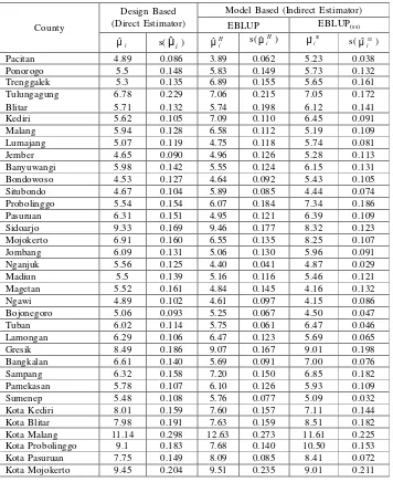
Model of small area estimation can be applied to estimate average of households expenditure per month for each of m = 37 counties in East Java, Indonesia. Data that be used in this case study are data of Susenas (National Economic and Social Survey, BPS) 2003 to 2005.

Table 1. Design Based and Model Based Estimates of County Means and Estimated Standard Error

County

Design Based (Direct Estimator)

Model Based (Indirect Estimator)

EBLUP EBLUP(ss)

i

µˆ s(

µ

ˆ

_i) µˆiH s( H i

µˆ ) ss

i

µˆ s( ss

i µˆ )

Pacitan 4.89 0.086 3.89 0.062 5.23 0.038

Ponorogo 5.5 0.148 5.83 0.149 5.73 0.132

Trenggalek 5.3 0.135 6.89 0.155 5.65 0.161

Tulungagung 6.78 0.229 7.06 0.215 7.05 0.172

Blitar 5.71 0.132 5.74 0.198 6.12 0.141

Kediri 5.62 0.105 7.09 0.110 6.45 0.091

Malang 5.94 0.128 6.58 0.112 5.19 0.109

Lumajang 5.07 0.119 4.75 0.118 5.74 0.081

Jember 4.65 0.090 4.96 0.126 5.28 0.113

Banyuwangi 5.98 0.142 5.55 0.124 6.15 0.131

Bondowoso 4.53 0.127 4.64 0.092 5.43 0.105

Situbondo 4.67 0.104 5.89 0.085 4.44 0.074

Probolinggo 5.54 0.154 6.07 0.184 7.34 0.186

Pasuruan 6.31 0.151 4.95 0.121 6.39 0.109

Sidoarjo 9.33 0.169 9.46 0.177 8.32 0.123

Mojokerto 6.91 0.160 6.55 0.135 8.25 0.107

Jombang 6.09 0.131 5.06 0.130 5.96 0.091

Nganjuk 5.56 0.125 4.40 0.041 4.87 0.029

Madiun 5.5 0.139 5.16 0.116 5.46 0.121

Magetan 5.52 0.161 4.84 0.145 4.16 0.132

Ngawi 4.89 0.102 4.61 0.097 4.15 0.086

Bojonegoro 5.06 0.093 5.25 0.067 4.50 0.047

Tuban 6.02 0.114 5.75 0.061 6.47 0.046

Lamongan 6.29 0.106 6.47 0.123 5.69 0.065

Gresik 8.49 0.186 9.07 0.167 9.01 0.198

Bangkalan 6.61 0.140 5.69 0.091 7.00 0.076

Sampang 6.32 0.158 7.20 0.150 6.85 0.182

Pamekasan 5.78 0.107 6.10 0.126 5.93 0.109

Sumenep 5.48 0.108 5.76 0.077 5.09 0.032

Kota Kediri 8.01 0.159 7.60 0.157 7.11 0.144

Kota Blitar 7.98 0.191 7.63 0.159 8.51 0.182

Kota Malang 11.14 0.298 12.63 0.273 11.61 0.225

Kota Probolinggo 9.1 0.183 7.68 0.140 10.50 0.153

Kota Pasuruan 7.75 0.149 8.09 0.085 8.41 0.072

[image:9.595.103.459.286.722.2]

(10)

885

County

Design Based (Direct Estimator)

Model Based (Indirect Estimator)

EBLUP EBLUP(ss)

i

µˆ s(

µ

ˆ

_i) µˆiH s( H i

µˆ ) ss

i

µˆ s( ss

i µˆ )

Kota Madiun 8.4 0.162 8.33 0.150 7.62 0.196

Kota Surabaya 11.45 0.328 11.81 0.353 11.16 0.321

Mean 0.149 0.138 0.124

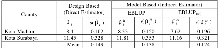
Table 1 reports the design based and model based estimates. The design based estimates is direct

estimator based on design sampling. EBLUP estimates,

H i µˆ

, use small are model with area effects (data

of Susenas 2005). Whereas, EBLUP(ss) estimates,

ss i µˆ

, use small are model with area and time effects

(data of Susenas 2003 to 2005). Estimated standard error denoted by s(

µ

ˆ

i_{), s(}

H i µˆ

), and s(

ss i µˆ

). It is clear from Table 1 that estimated standard error mean of model based is less than design based. The estimated standard error mean of EBLUP(ss) is less than EBLUP.

8.

Conclusion

Small area estimation can be used to increase the effective sample size and thus decrease the standard error. For such repeated surveys considerable gain in efficiency can be achieved by borrowing strength across both small area and time. Availability of good auxiliary data and determination of suitable linking models are crucial to the formation of indirect estimators.

9.

Reference

Datta, G.S, and Lahiri, P. (2000). A Unified Measure of Uncertainty of Estimated Best Linear Unbiased

Predictors (BLUP) in Small Area Estimation Problems, Statistica Sinica, 10, 613-627.

Pfeffermann, D. (2002). Small Area Estimation – New Developments and Directions. International

Statistical Review, 70, 125-143.

Pfeffermann, D. and Tiller, R. (2006). State Space Modelling with Correlated Measurements with Aplication to Small Area Estimation Under Benchmark Constraints. S3RI Methodology Working

Paper M03/11, University of Southampton. Available from: http://www.s3ri.soton.ac.uk/

publications.

Rao, J.N.K. (2003). Small Area Estimation. John Wiley & Sons, Inc. New Jersey.

Rao, J.N.K., dan Yu, M. (1994). Small Area Estimation by Combining Time Series and Cross-Sectional

Data. Proceedings of the Section on Survey Research Method. American Statistical Association.

Swenson, B., dan Wretman., J.H. (1992). The Weighted Regression Technique for Estimating the

Variance of Generalized Regression Estimator. Biometrika, 76, 527-537.

Thompson, M.E. (1997). Theory of Sample Surveys. London: Chapman and Hall.

[image:10.595.100.458.108.190.2]