Haze Removal Concept in Remote Sensing.

http://dx.doi.org/10.12988/ams.2016.6128

Haze Removal Concept in Remote Sensing

Asmala Ahmad

Department of Industrial Computing

Faculty of Information and Communication Technology Universiti Teknikal Malaysia Melaka

Melaka, Malaysia

Shaun Quegan

Department of Applied Mathematics School of Mathematics and Statistics

University of Sheffield Sheffield, United Kingdom

Copyright © 2016 Asmala Ahmad and Shaun Quegan. This article is distributed under the Creative Commons Attribution License, which permits unrestricted use, distribution, and reproduction in any medium, provided the original work is properly cited.

Abstract

Atmospheric haze causes visibility to drop, therefore affecting data acquired using optical sensors on board remote sensing satellites. Haze modifies the spectral signatures of land cover classes and reduces classification accuracy so causing problems to users of remote sensing data. This paper addresses general concepts of haze removal from remote sensing data. Degradation of satellite data is caused by two key components, i.e. haze scattering and signal attenuation. In developing the concept, a statistical model that makes use both components is used. The former is represented by a weighted haze mean while the latter is represented by a haze randomness component that deals with the signal attenuation. The results show that haze scattering can be removed by subtracting an estimated weighted haze mean while signal attenuation can be removed by applying a spatial filter.

Keywords: Haze, Remote Sensing, Classification Accuracy

1 Introduction

Haze modifies the spectral signatures of land classes [1], [8], [9], [16] and reduces classification accuracy [2], [18], [19] so causing problems to users of remote

useful-ness of the data [12]. In [10], we modelled hazy satellite data as

 



 1

 



 2

 

i i i O i i

L V  1 V T L + V H , where,L V , _i

 

T , _i H , _i _i 1

 

V ,

 2

 

i V

 , L and _O V are the true signal component, the pure haze component, the signal attenuation factor, the haze weighting, the radiance scattered by the atmosphere and the visibility for band i. From this equation, it is clear that the degradation of hazy satellite data is caused by haze scattering and signal attenuation characterised by _i 2

 

V and _i 1

 

V respectively. Ideally, to reduce the haze effects and restore the surface information, we need to reduce the former so that _i 2

 

V H_i 0 and restore the latter so that



1_i 1

 

V



T_i T_i. In practice, the effects of signal attenuation through _i 1

 

V are not significant, so their removal is not important. On the other hand, the effects of _i 2

 

V H_i is very significant; therefore, this paper is concerned mainly with reducing_i 2

 

V H_i. Since the primary issue is to develop haze removal, we need to define physical processes for removing haze. Section 2 clarifies the concepts of haze removal and mathematically analyses these processes, and in Section 3, the haze removal methods are described.

2 General Concepts of Haze Removal

In [10], we developed a statistical model for hazy satellite data, which can be expressed as:

 



 1

 



 2

 

i i i O i i

L V  1 V T L + V H (1)

where , T ,_i , L , _O _i 1

 

V and  _i2

 

V are the hazy dataset, the signal component, the pure haze component, the radiance scattered by the atmosphere, the signal attenuation factor and the haze weighting in satellite band ,

respectively. H can be expressed as: _i

v

i i i

H =H H (2)

Where H is the haze mean, which is assumed to be uniform within the image or _i sub-region of the image, and

v

i

H is a zero-mean random variable corresponding to haze randomness. Hence:

 

i_v

 

i

So Equation (1) can be written as:

 

 

 

 

 

v

1 2

i i i O i i i

L V  _1 V _T +L  V _H H _ (4) In order to remove the haze effects [5], [6], [14], [15] we need to remove both the weighted haze mean  _i2

 

V H_iand the varying component  

 

v

2

i V Hi

 and deal

with the signal attenuation factor  _i1

 

V .

From [7], the effects of  _i1

 

V to classification accuracy are not significant, so we will not consider their removal throughout the analysis. We normally do not have prior knowledge about  _i2

 

V H_i therefore we need to estimate it from the hazy data itself. If the estimate is  _i2

 

V H_i, subtracting it from L V yields: _i

 

 

 

 

 

 

 

 

 

 

 

Z v

2 1 2

i i i i i i O i i i

2

i i

L V L V V H 1 V T L V H H

V H

   

   _{ }   _  _



+

(5)

Equation (5) becomes:

 

 

 

 

 

 

 

 

 

Z v

1 2 2 2

i i i i i i i i i O

L V  _1 V _T _ V H  V H _  V H L

 

+ (6)

where __i 2

 

V H_i_i 2

 

V H_i_

  is the error associated with the difference

between the ideal and estimated weighted haze mean. The haze randomness component  

 

v

2

i V Hi

 can then be smoothed by applying a spatial filter:

 



_Z

 



i i

f V h L V (7)

where h is the filter function and f Vˆ

 

is the restored data. Note that this also smoothes the signal component; we will show later that filtering is only necessary for thick haze where the haze variability is much greater than the surface. For thin haze, the surface variability is much greater than the haze; filtering causes degradation to the surface and therefore is not required.

 



 



 

 

 

 

 

 

 

 

 

 

 

 

 

 



 

 





 

 



 

 

 

Z v v

i linear i

1 2 2

i linear i linear i i i i

2

i linear i linear O

1 2 2

i linear i linear i i linear i i

2

i linear i O

f V h L V

1 β V h T h β V H β V H

β V h H h L

1 β V h T h β V H h β V H

β V h H L

      _{  }  _         _{ }    + + (8)

Linear filters are usually normalised to 1 i.e the sum of the filter coefficients is 1; since the haze mean H is assumed to be constant, hence: _i

 

 

 

 

 

 



 

 



 

 

 

v

1 2 2

i i linear i i i linear i i

2

i linear i O

f V 1 β V h T β V H h β V H

β V h H L

 

 _{ }  

 +

(9)

The median filter is non-linear, so this separation is not possible:

 



 



 

 

 

 

 

 

 

 

Z

v

i Median i

1 2 2

i i i i i i

2

i i O

f V h L V

1 β V T β V H β V H

Median

β V H L

 _{  }  _ _   _ _   _{ }  _   

+ (10)

For an ideal case where the haze mean is known exactly, β _i2

 

V H β_i   _i2

 

V H_i , so the degraded data after subtracting the haze mean becomes:

 

 

 

 





 

 

v Z ideal 1 2

i i i i i O

L V  1 V T + V H L (11)

Consequently, when using average and Gaussian filters, we have:

 

 



 

 



 

 

 

 

 

 

Z ideal Z ideal

v

i linear i

1 2

i linear i i linear i O

f V h L V

1 V h T V h H L



 

 _{ } + 

(12)

 

 



 

 



 

 

 

 





Z ideal Z ideal

v

i Median i

1 2

i i i i O

f V h L V

Median 1 V T V H L



 

 _  _ + 

(13)

From Equation (12), it is clear that a linear filter filters not only the haze randomness

v

i

H , but also the surface information T . For thin haze (i.e. small _i

 1

 

i V

 and  _i2

 

V ), filtering will cause degradation to T . For thick haze, we _i have big  _i1

 

V and  _i2

 

V ; the effect of filtering to

v

i

H is more significant than T . Although small, _i _1 _i1

 

V _h_linear

 

T_i , the structure of



 _i



and C in T is still preserved and therefore will be useful for classification purpose [3], _i [4], [18].

For non-linear filters such as median filtering (Equation (13)), the filtering affects the linear summation of the signal and haze components as a whole, i.e.

 

 

 

 



v



1 2

i i i i O

Median 1_  V _T + V H L . For thick haze, the input of median filtering is dominated by

v

i

H ; therefore, the effects of haze will be reduced to some extent. For thin haze, the input of the filtering dominated by T ; therefore, _i degradation of surface occurs.

Based on this analysis, haze removal consists of (a) estimating the haze mean from hazy data using (pseudo invariant features) PIFs, (b) subtracting the haze mean from the data in order to remove the haze path radiance and (c) applying spatial filtering in order to reduce the haze randomness within the data.

3 Methods

To test the haze removal procedures, we first make use of the simulated hazy datasets, for which the visibilities and values of  _i2

 

V H_i are known. The assumptions are:

(a) The haze is spatially uniform.

(b) The haziness within the data is mainly associated with additive effects due to scattering from particles; therefore, most of the efforts done here are to deal with the haze scattering term  _i2

 

V H_i.

3.1 Estimation of Haze Mean Radiance

In order to estimate  _i2

 

V H_i, we first need to establish relationships between the exact  _i2

 

V H_i and the corresponding PIF radiances within the simulated hazy datasets for different levels of visibility. In equatorial countries such as Malaysia, only a small amount of variation occurs in bidirectional reflectance distribution function (BRDF) throughout a year, so their effects on the target radiance for different acquisition dates are assumed to be negligible. Variation in PIF spectral radiance from multi-date datasets is therefore assumed to be due to only atmospheric conditions, i.e. signal attenuation and haze scattering [5].

The study area (Klang, Selangor) is located within a flat region, near the west coast of Malaysia. The PIF pixels are chosen from rooftops of terrace houses, which are not too high and covers about 44% of Malaysian houses [17]. The typical area of this type of houses is about 20 feet in wide and 70 feet in length, with built-up area of about 1200 square feet while the remaining area is garden. Most of these houses were built using clay bricks and have clay roof tiles [17]. The houses are usually built in rows that are separated by roads made of tarmac. Therefore, it is clear that most of the housing areas are covered with impervious surfaces and have very little vegetation; therefore are little affected by biological changes [11]. In sub urban region, such housing area normally surrounded by distinct features such as rubber and oil palm plantation. It is important to note that in order to minimised mixed pixel problem, the PIF should have at least a few pixels in size [13] so that measurement made from a satellite instantaneous field of view (IFOV) (i.e. 30 m by 30 m for Landsat) will not fall out of the chosen features. In practice mixed pixel problem in PIF is unavoidable, however, this was minimised because the objects within a single PIF pixel are mostly impervious surfaces (clay bricks and tiles and tarmac). A schematic diagram on what is in a PIF pixel is illustrated in Figure 1.

(a) (b)

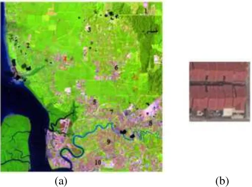
[image:6.595.139.486.557.714.2]

For visibilities from 18 km to 2 km, ten PIFs that are distributed throughout the image were selected and their radiances were extracted. Figure 2 (a) shows Landsat bands 4, 5 and 3 assigned to red, green and blue channels from 11 February 1999 for Klang, in Selangor, Malaysia. The white box indicates the location of the PIFs which are indicated by the red squares.

Fig (b) shows the enlarged version of PIF number 7. The PIFs are selected from the rooftops of houses that have nearly constant radiances. It can be seen that the PIF consists of house rooftops and roads, with little vegetation.

(a) (b)

Fig. 2: (a) Landsat bands 5, 4 and 3 assigned to red, green and blue channels from 11 February 1999 for Klang, in Selangor, Malaysia. (b) Enlarged version of PIF

number 7 taken from Google Maps

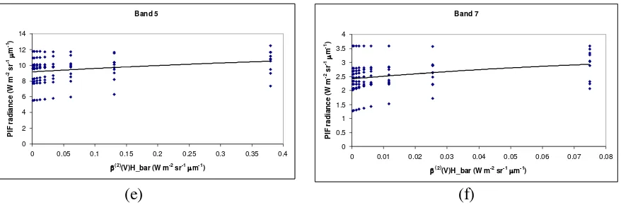
Scatterplots of  _i2

 

V H_i versus the PIF radiance, for bands 1, 2, 3, 4, 5 and 7 are plotted in Figure 3. The PIF radiance values are indicated by ‘’. The PIF radiance increases steadily as  _i2

 

V H_i gets larger (i.e. haze gets thicker) due to the increasing atmospheric effects (haze scattering and signal attenuation). Hence, by knowing the radiances of the PIF pixels, it is possible to predict the corresponding  _i2

 

V H_i . In order to do so, we carried out regression between

 2

 

i V Hi

 and the PIF radiance. The solid curves in Figure 3 are the regression curves which represent the predicted  _i2

 

V H_i, i.e.  _i2

 

V H_i. It can be seen that the regression curves for all the bands have similar trends and therefore can be modelled by the same regression equation:  

 

 

i i

2 2

i V H1 a LPIF bLPIF c

    ,

where a, b, and c are the regression variables and i

PIF

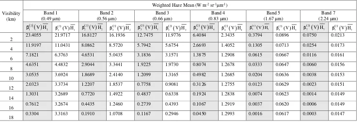
[image:7.595.172.426.266.454.2]

The regression variables, a, b, and c and the coefficient of determination, R2, are given in Table 1. Overall the R2 _{values are greater than 0.9, indicating a good fit}

between the regression curve and the data in all the bands. The estimated weighted haze mean radiance  _i2

 

V H_i for visibilities 2 to 18 km, calculated using the regression equation, is given in Table 2. In this table, the ideal weighted haze mean radiance  _i2

 

V H_i is also given for comparison. Bands with shorter wavelengths possess larger

i

PIF

L and

 2

 

i V Hi

 values due to the greater haze scattering than longer wavelengths. There is a sharper increase in

i

PIF

L in bands with shorter wavelengths (bands 1, 2 and 3) compared to those with longer wavelengths (bands 4, 5 and 7), indicated that the former are affected by haze while the later almost not being affected by haze. It is clear that bands with shorter wavelengths have larger

i

PIF

L , therefore brighter PIFs, than clear or less hazy image. Bands with longer wavelengths have a somewhat constant

i

PIF

L , indicating that haze has almost not effects on the PIFs.

Band 1 40 50 60 70 80 90 100 110 120 130

0 5 10 15 20 25

(2)_{(V)H_bar (W m}-2 _sr-1 _m-1₎

P IF r a d ia n c e ( W m

-2 s

r -1  m -1) Band 2 0 20 40 60 80 100 120 140 160

0 5 10 15 20

(2)_{(V)H_bar (W m}-2 _sr-1 _m-1₎

P IF r a d ia n c e ( W m

-2 s

r

-1



m

-1)

(a) (b)

Band 1 0 20 40 60 80 100 120 140

0 2 4 6 8 10 12 14

(2)_{(V)H_bar (W m}-2 _sr-1 _m-1₎

P IF r a d ia n c e ( W m

-2 s

r -1  m -1) Band 4 0 10 20 30 40 50 60 70 80 90

0 1 2 3 4 5 6 7

(2)_{(V)H_bar (W m}-2 _sr-1 _m-1₎

P IF r a d ia n c e ( W m

-2 s

r

-1



m

-1)

Band 5 0 2 4 6 8 10 12 14

0 0.05 0.1 0.15 0.2 0.25 0.3 0.35 0.4

(2)_{(V)H_bar (W m}-2 _sr-1 _m-1₎

P IF r a d ia n c e ( W m

-2 s

r -1  m -1) Band 7 0 0.5 1 1.5 2 2.5 3 3.5 4

0 0.01 0.02 0.03 0.04 0.05 0.06 0.07 0.08

(2)_{(V)H_bar (W m}-2 _sr-1 _m-1₎

P IF r a d ia n c e ( W m

-2 s

r

-1



m

-1)

[image:9.595.89.528.139.284.2]

(e) (f)

Fig. 3: Regression analysis, of PIF radiance from the simulated hazy data against _i2

 

V H_i, for (a) band 1, (b) band 2, (c) band 3, (d) band 4, (e) band 5

and (f) band 7. The corresponding regression equations are in Table 1.

Table 1: Regression model to predict  _i2

 

V H_i for bands 1, 2, 3, 4, 5, and 7;

PIF

L is the PIF radiance

Band Regression Model R2

1  

 

 

1 1

2 2

1 V H1 0.0023* LPIF 0.7176*LPIF 29.397

     0.9956

2  

 

 

2 2

2 2

2 V H2 0.0011* LPIF 0.3771*LPIF 13.103

     0.9539

3  

 

 

3 3

2 2

3 V H3 0.001* LPIF 0.334* LPIF 9.8765

     0.9395

4  

 

 

4 4

2 2

4 V H4 0.0041* LPIF 0.3157*LPIF 6.8741

    0.1827

5  

 

 

5 5

2 2

5 V H5 0.0046* LPIF 0.0647*LPIF 0.2629

    0.0788

7  

 

 

7 7

2 2

7 V H7 0.0028* LPIF 0.0026*LPIF 0.0021

[image:10.842.54.803.165.418.2]

Table.2: Comparison between  _i2

 

V H_i (exact) and  _i2

 

V H_i (estimated)

Visibility (km)

Weighted Haze Mean (W m-2 _sr-1_m-1₎

Band 1 (0.49 m)

Band 2 (0.56 m)

Band 3 (0.66 m)

Band 4 (0.83 m)

Band 5 (1.67 m)

Band 7 (2.24 m)  2

 

1 V H1

  2 _{ }

1 V H1

  2  

2 V H2

  2 _{ }

2 V H2

  2  

3 V H3

  2 _{ }

3 V H3

  2  

4 V H4

  2 _{ }

4 V H4

  2  

5 V H5

  2 _{ }

5 V H5

  2  

7 V H7

  2 _{ }

7 V H7



4 Restoration of Surface Information Using Spatial Filtering

After subtracting the estimated haze mean component, the haze noise within the image is expected to behave as a zero-mean random variable associated with haze randomness,  

 

v

2

i V Hi

 (see Equation (7)) (although errors in the haze mean estimate will cause a bias). If we assume the estimate of  _i2

 

V H_i is good enough that can be neglected, our concern now is to reduce  

 

v

2

i V Hi

 by using

spatial filtering. Here, three types of filtering are considered, i.e. average, median and Gaussian.

4.1 Average Filter

The main advantages of average filtering are that it is simple, intuitive and easy to use, but still effective in reducing noise. Average filtering simply replaces each pixel value in an image with the average value of its neighbours, including itself. The average filter depends on the size of the window used, and the size can be increased to suit the severity of the haze.

4.2 Gaussian Filter

A continuous Gaussian filter has the form:

 

 

2 2 2

x y 2σ

g 2

1

h x, y e

2πσ

 

 (14)

where x and y are distance from the origin in the horizontal and vertical direction respectively and  is the standard deviation of the Gaussian filter. In order to preserve the mean energy in the digital case, the form shown in Equation (14) is normalised by the sum of the filter coefficients, to give:

 

 

 

g N M

2 2 g M N r ₂s ₂

h r,s

h r,s

h r,s

 

 



 

(15)

During filtering, the centre pixel receives the heaviest weight, and pixels receive smaller weights as the distance from the window centre increases. We use built-in Gaussian filters in the ENVI image processing software, in which σ is related to window size by σ M

8

 for an M M _{window. Plots of the 1-dimensional}

the original image. On the other hand, the 21 x 21-window gives much lower weighting across the filter (the highest is 0.02 and lowest is nearly 0) so is likely to resemble an average filter.

-100 -9 -8 -7 -6 -5 -4 -3 -2 -1 0 1 2 3 4 5 6 7 8 9 10 0.1

0.2 0.3 0.4 0.5 0.6 0.7 0.8 0.9 1

W

e

ig

h

ti

n

g

Location

Weighting Vs. Location within A Gaussian Filter Window

[image:12.595.185.409.185.369.2]

3 x 3 5 x 5 7 x 7 11 x 11 21 x 21

Fig. 4: Distribution of pixel weighting for 3 by 3, 5 by 5, 7 by 7, 11 by 11 and 21 by 21 window sizes, of a Gaussian filter in 1-dimension

(a) (b) (c)

Fig. 5: Gaussian filter (a) 3 by 3, (b) 5 by 5 and (c) 21 by 21 but only part of centre cells

4.3 Median Filter

Median filtering is often used to remove noise from a degraded image and at the same time preserve edges. It replaces the central pixel with the median value in the window. A similar approach to that for average and Gaussian filtering is used to determine the best window size for a specific visibility.

5 Conclusion

and therefore need to be dealt in order to remove haze. Hence, the haze removal needs to undergo weighted haze mean estimation and subtraction, and spatial filtering.

Acknowledgements. We would like to thank Universiti Teknikal Malaysia Melaka (UTeM) for funding this study under the Malaysian Ministry of Higher Education Grant (FRGS/2/2014/ICT02/FTMK/02/F00245).

References

[1] A. Ahmad and M. Hashim, Determination of Haze API From Forest Fire Emission During the 1997 Thick Haze Episode in Malaysia using NOAA AVHRR Data, Malaysian Journal of Remote Sensing and GIS, 1 (2000), 77 - 84.

[2] A. Ahmad and S. Quegan, Analysis of maximum likelihood classification on multispectral data, Applied Mathematical Sciences, 6 (2012), 6425 - 6436.

[3] A. Ahmad and S. Quegan, Analysis of maximum likelihood classification technique on Landsat 5 TM satellite data of tropical land covers, Proceedings of 2012 IEEE International Conference on Control System, Computing and

Engineering, (2012), 280 - 285.

http://dx.doi.org/10.1109/iccsce.2012.6487156

[4] A. Ahmad and S. Quegan, Comparative analysis of supervised and unsupervised classification on multispectral data, Applied Mathematical

Sciences, 7 (2013), no. 74, 3681 - 3694.

http://dx.doi.org/10.12988/ams.2013.34214

[5] A. Ahmad, S. Quegan, et al., Haze reduction from remotely sensed data,

Applied Mathematical Sciences, 8 (2014), no. 36, 1755 - 1762.

http://dx.doi.org/10.12988/ams.2014.4289

[6] A. Ahmad and S. Quegan, The Effects of haze on the spectral and statistical properties of land cover classification, Applied Mathematical Sciences, 8

(2014), no. 180, 9001 - 9013. http://dx.doi.org/10.12988/ams.2014.411939 [7] A. Ahmad and S. Quegan, The Effects of haze on the accuracy of satellite

[8] A. Ahmad, Analysis of Landsat 5 TM data of Malaysian land covers using ISODATA clustering technique, Proceedings of the 2012 IEEE Asia-Pacific

Conference on Applied Electromagnetic (APACE 2012), (2012), 92 - 97.

http://dx.doi.org/10.1109/apace.2012.6457639

[9] A. Asmala, M. Hashim, M. N. Hashim, M. N. Ayof and A. S. Budi, The use of remote sensing and GIS to estimate Air Quality Index (AQI) Over Peninsular Malaysia, GIS Development, (2006), 5.

[10] A. Ahmad and S. Quegan, Haze modelling and simulation in remote sensing satellite data, Applied Mathematical Sciences, 8 (2014), no. 159, 7909 - 7921. http://dx.doi.org/10.12988/ams.2014.49761

[11] J. R. Schott, C. Salvaggio and W. Volchok, Radiometric scene normalization using pseudoinvariant features, Remote Sensing of

Environment, 26 (1988), 1 - 16.

http://dx.doi.org/10.1016/0034-4257(88)90116-2

[12] C. Y. Ji, Haze reduction from the visible bands of LANDSAT TM and ETM+ images over a shallow water reef environment, Remote Sensing of

Environment, 112 (2008), 1773 - 1783.

http://dx.doi.org/10.1016/j.rse.2007.09.006

[13] D. G. Hadjimitsis, C. R. I. Clayton and A. Retalis, The use of selected pseudo-invariant targets for the application of atmospheric correction in multi-temporal studies using satellite remotely sensed imagery,

International Journal of Applied Earth Observation and Geoinformation,

11 (2009), no. 3, 192 - 200.

http://dx.doi.org/10.1016/j.jag.2009.01.005

[14] G. D. Moro and L. Halounova, Haze removal for high-resolution satellite data: a case study, Int. J. of Remote Sensing, 28 (2007), no. 10, 2187 - 2205. http://dx.doi.org/10.1080/01431160600928559

[15] M. F. Razali, A. Ahmad, O. Mohd and H. Sakidin,

N. I. S. Bahari,

Quantifying haze from satellite using haze optimized transformation (HOT), Applied Mathematical Sciences, 9 (2015), no. 29, 1407 - 1416. http://dx.doi.org/10.12988/ams.2015.5130

[16] M. Hashim, K. D. Kanniah, A. Ahmad, A. W. Rasib, Remote sensing of tropospheric pollutants originating from 1997 forest fire in Southeast Asia,

Asian Journal of Geoinformatics, 4 (2004), 57 - 68.

thermal heat storage in building facade, Sustainability, 2 (2010), no. 8, 2365 - 2381. http://dx.doi.org/10.3390/su2082365

[18] M. Story and R. Congalton, Accuracy assessment: a user's perspective,

Photogrammetric Engineering and Remote Sensing, 52 (1986), 397 - 399.

[19] U. K. M. Hashim and A. Ahmad, The effects of training set size on the accuracy of maximum likelihood, neural network and support vector machine classification, Science International-Lahore, 26 (2014), no. 4, 1477 - 1481.