Covariance structure analysis of regiona

Covariance Structure Analysis of Regional Development Data: An

Application to Municipality Development Assessment

†

Dario Czirákya,*, Jakša Puljizb, Krešimir Jurlinb, Sanja Malekovićb, Mario Polićb a

Department for Resource Economics, IMO

b

Department for International Economic Relations, IMO IMO, 2 Farkaša-Vukotinovića, 10000 Zagreb, Croatia

___________________________________________________________________________

Abstract

This paper proposes a multivariate statistical approach based on covariance structure analysis for assessment of the regional development level with an application to development ranking of 545 Croatian municipalities. Municipality-level data ware collected on economic, structural, and demographic dimensions and preliminary factor and principal component analysis were computed to analyse empirical groupings of the variables. Next, confirmatory factor analytic models were estimated with the maximum likelihood technique and subsequently their implied structure was formally tested. Testing was extended to a joint model including all three dimensions (economic, structural and demographic) and their covariance structure was modelled with a recursive structural equation model. Finally, scores were estimated for latent variables thereby allowing (i) estimation of the latent development level of the territorial units, (ii) ranking of all units on an interval scale in respect to their latent development level, and (iii) selection of a given percentage of units for inclusion into special state-care subsidy programme.

JEL Classification: R1, C3, C1

Keywords: Regional development; Covariance structure analysis; Multivariate methods;

Factor analysis; Structural equation modelling; Latent variables

___________________________________________________________________________

1. Introduction

Regional development assessment is a methodologically challenging and policy relevant issue. Aside from purely academic investigation into geo-economic and social patterns and groupings of regional units, there is an important policy requirement for estimating the level

†

Paper presented at 42nd Congress of the European Regional Science Association, Dortmund, Germany, August 27 – 31, 2002.

‡

of regional development for the purpose of development classification and funding considerations. The Structural Funds of the European Union provide one such example where the level of economic development (approximated by the GDP per capita), in principle, determines the inclusion or exclusion of particular European regions into the regional financial schemes allocations.

In this paper we present a multivariate statistical framework for assessment of the regional development level developed for the purpose of ranking 545 Croatian municipalities. The statistical model was needed to identify municipalities lacking in development. A given percentage of the most underdeveloped municipalities was planned to be subsequently included into a regional funding scheme financed from the national budget. This paper presents the results from the second phase of the project “Criteria for the Development Level Assessment of the Areas Lagging in Development” that was carried out by the IMO for the Croatian Ministry of Public Works (Maleković, 2001). The purpose of the project was to provide an analytical base for evaluation of the development level of the Croatian territorial units (municipalities) with an aim of widening the span of territorial units which are currrently receiving state support under the “Law on Areas of Specific Governmental Concern”. The results of the analysis were intended to serve as the basis for changing the approach to defining and supporting the development of areas of special state concern. Unlike the former approach, whose sole criterion has been whether an area was war-affected (i.e., under Serbian occupation in the 1991-1995 war), the new approach defines economic, structural, and

demographic criteria (dimensions), as well as a combination of indicators and choice

procedures with an aim of obtaining a better quality development evaluation.

There are some important aspects that have substantially influenced our approach. First, the unit of analysis is municipality and that fact has resulted in some major problems, mostly regarding the availability and a quality of the data. Second is the policy relevance and a political sensitivity of the whole project. Namely, in the situation when direct result of the project is a list of municipalities eligible to enter “Areas of Special State Concern” which results in their privileged status concerning state subsidies, tax deductions, etc., the proposed solution needed to be maximally transparent and unambiguous, and a space left for political manipulations has to be minimised.

1994) proposed the use of a co-plot technique for the study of regional disparities. Multidimensional scaling techniques (Borg and Groenen, 1997), metric scaling (Weller and Romney, 1990) and correspondence analysis (Greenacre, 1993; Greenacre and Blasius, 1994; Blasius and Greenacre, 1998) can be also used to investigate clustering and grouping of territorial units. Most of these methods minimise some metric or not metric criteria in respect to given variables thereby allowing proximity groupings of units and/or variables. However, it is often the case that the applied model selection criteria are to a large degree arbitrary and subject to “fine-tuning” and data mining. At best such grouping techniques offer broad geographical picture of similarity clusters, i.e., territorial units that are more similar among themselves than with the rest of the units. Moreover, clustering and grouping techniques do not offer justification for exclusion decision, namely, if an “underdeveloped” cluster is defined so to include more units that can be funded from the subsidiary funds, there are no grounds for exclusion of some members of that cluster as they do not posses a unique “development score”.

In cases such as ours clear universal criteria and transparent models are needed. Furthermore, it is often necessary to estimate the underlying (i.e., latent) development level for each territorial unit, not merely classify them into separate clusters and then substantively interpret these clusters as more or less developed.

2. Regional development data

The data for the analysis came from several Croatian sources such as the Ministry of finance, the Health Insurance Institute, and the Statistical Bureau. The collected data is on the municipality level and presents lowest aggregation level available in Croatia. We were able to collect data on 11 indicators, roughly grouped into economic, structural and demographic

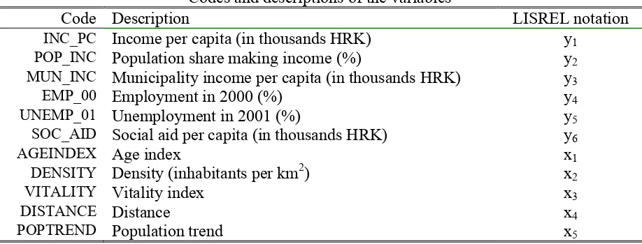
dimensions. These broad categories are defined on substantive grounds and are later analysed by the means of exploratory and confirmatory factor analysis to check their empirical similarity patterns. The economic indicators generally included income-type variables, namely income per capita, share of population earning income and municipality (direct) income. The structural indicators were essentially employment measures such as employment percentage (we used the 2000 data), unemployment percentage (using 2001 data) and social aid per capita. Data from different years were used due to availability of more reliable employment indicators for the year 2000. Demographic indicators included the age index (defined as the number of people older then 65 divided by the number of people younger then 20), density (defined as the number of inhabitants per square kilometre), vitality (number of live births per 100 births), distance (time in minutes needed to reach the County centre by car) and population trend (total municipality population in 2001 over total population in 1991). The codes and brief description are shown in Table 1. We also include the LISREL notation (see Jöreskog, et al., 2000) that will be used in later analysis in the third column.

Table 1

Codes and descriptions of the variables

Code Description LISREL notation

INC_PC Income per capita (in thousands HRK) y1

POP_INC Population share making income (%) y2

MUN_INC Municipality income per capita (in thousands HRK) y3

EMP_00 Employment in 2000 (%) y4

UNEMP_01 Unemployment in 2001 (%) y5

SOC_AID Social aid per capita (in thousands HRK) y6

AGEINDEX Age index x1

DENSITY Density (inhabitants per km2) x2

VITALITY Vitality index x3

DISTANCE Distance x4

POPTREND Population trend x5

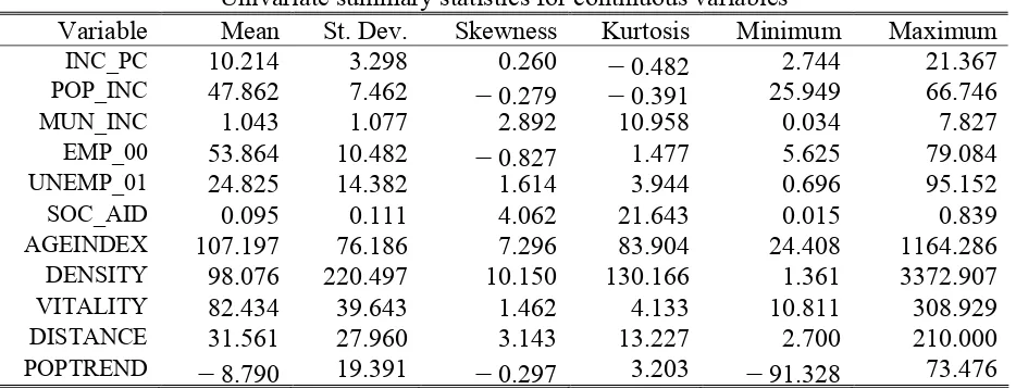
DENSITY variable. DENSITY has higher variance because it is expressed in the original metric without rescaling while most other variables were expressed either in thousands or in percentages. We left the population density variable in people per square kilometre units because we could find no meaningful rescaling that could be justified on substantive grounds. Consequently, we note that DENSITY has greater relative variance then any other variable in the analysis. The issue of removing differences in variances across variables through standardisation is a rather debated one. Some authors base their entire analysis on standardised variables (e.g., Soares et al., 2002) which amounts to analysing correlation matrices instead of covariance matrices in all subsequent econometric models (see Gerbing and Anderson, 1984).

Table 2

Univariate summary statistics for continuous variables

Variable Mean St. Dev. Skewness Kurtosis Minimum Maximum

INC_PC 10.214 3.298 0.260 -_0.482 2.744 21.367

POP_INC 47.862 7.462 -_0.279 -_0.391 25.949 66.746

MUN_INC 1.043 1.077 2.892 10.958 0.034 7.827

EMP_00 53.864 10.482 -_0.827 1.477 5.625 79.084

UNEMP_01 24.825 14.382 1.614 3.944 0.696 95.152

SOC_AID 0.095 0.111 4.062 21.643 0.015 0.839

AGEINDEX 107.197 76.186 7.296 83.904 24.408 1164.286

DENSITY 98.076 220.497 10.150 130.166 1.361 3372.907

VITALITY 82.434 39.643 1.462 4.133 10.811 308.929

DISTANCE 31.561 27.960 3.143 13.227 2.700 210.000

POPTREND -_8.790 19.391 -_0.297 3.203 -_91.328 73.476

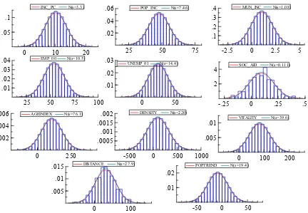
However, our methodology is mainly based on the analysis of covariance rather then correlation structures thus we preserve the original metrics of the variables (at least up to the point of substantive interpretability).

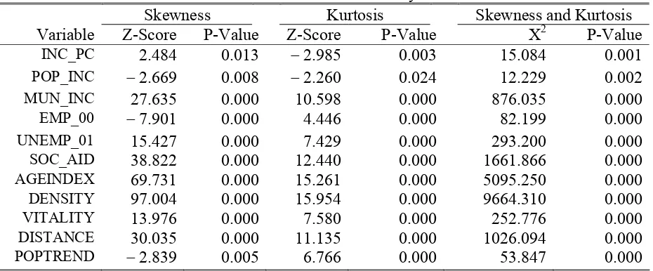
We note that certain multivariate techniques yield identical results regardless of which covariance matrix is analysed, however in general the standards errors and overall fit statistics can be wrong if the correlation matrix is analysed in place of the covariance matrix (see Cudek, 1989; Jöreskog, 2001: 209-214). We proceed with formal univariate and multivariate normality tests (D’Agostino, 1986; Doornik and Hansen, 1994; Mardia, 1980). The results of the normality tests are shown in Table 3.

D’Agustino (1970; 1971), Bowman and Shenton (1975), Shenton and Bowman (1977) and Belanger and D’Agostino (1990).

0 10 20

.05 .1

INC _ PC N(s=3 .3 )

20 40 60

.025 .05

POP_ INC N(s=7 .4 6 )

0 5

.5 1

MUN_ INC N(s=1 .0 8 )

0 25 50 75 .02

.04

EMP_ 0 0 N(s=1 0 .5 )

0 50 100

.02 .04

UNEMP_ 0 1 N(s=1 4 .4 )

0 .5 1

2.5 5 7.5

10 SOC _ AID N(s=0 .1 1 1 )

0 500 1000 .005

.01

AGEINDEX N(s=7 6 .1 )

0 1000 2000 3000 .0025

.005 .0075

.01 DENSITY N(s=2 2 0 )

0 100 200 300 .005

.01

.015 VITALITY N(s=3 9 .6 )

0 100 200 .01

.02

.03 DISTANC E N(s=2 7 .9 )

-100 0 100

.01 .02 .03

.04 POPTR END N(s=1 9 .4 )

Figure 1. Empirical density (Gaussian kernel estimate): original data

Table 3

Tests of univariate normality*

Skewness Kurtosis Skewness and Kurtosis

Variable Z-Score P-Value Z-Score P-Value X2 P-Value

INC_PC 2.484 0.013 -2.985 0.003 15.084 0.001

POP_INC _-2.669 0.008 -2.260 0.024 12.229 0.002

MUN_INC 27.635 0.000 10.598 0.000 876.035 0.000

EMP_00 -7.901 0.000 4.446 0.000 82.199 0.000

UNEMP_01 15.427 0.000 7.429 0.000 293.200 0.000

SOC_AID 38.822 0.000 12.440 0.000 1661.866 0.000

AGEINDEX 69.731 0.000 15.261 0.000 5095.250 0.000

DENSITY 97.004 0.000 15.954 0.000 9664.310 0.000

VITALITY 13.976 0.000 7.580 0.000 252.776 0.000

DISTANCE 30.035 0.000 11.135 0.000 1026.094 0.000

POPTREND -2.839 0.005 6.766 0.000 53.847 0.000

* The normality tests were computed with PRELIS 2 (Jöreskog and Sörbom, 1996).

techniques which are rather sensitive to departures from normality. Consequently, in section 3.3 we will attempt to normalise these variables using monotonic transformation techniques.

3. Econometric methodology

3.1. Multivariate modelling

Multivariate methods used in regional development research generally fall into variable classification (e.g., factor analysis) or classification of cases techniques (e.g. cluster analysis, Q-factor analysis). The two classes of techniques could be also combined. For example, Soares, et al. (2002) first perform factor analysis on the variables and then they cluster the cases (i.e., territorial units) using cluster analysis on the original variables as well as on the factor scores. This approach of searching for general patterns of similarities also underlines other similar space-proximity methods such as the co-plot technique (Lipshitz and Raveh 1998; 1994), multidimensional scaling (Borg and Groenen, 1997), metric scaling (Weller and Romney, 1990) and correspondence analysis (Greenacre, 1993; Greenacre and Blasius, 1994; Blasius and Greenacre, 1998). However, nether of these techniques allows estimation of the development level of territorial units on a single scale (preferably interval) nor do they allow ranking of all analysed units in respect to some uniquely defined development criteria. The trouble is that these criteria are at the heart of the problem we need to solve in the first place. Consequently, we need to design an alternative methodological framework within which we can achieve given objectives of comparative development evaluation and ranking of all units. Our proposed solution is to model the covariance structure of the municipality socio-economic and demographic data within the class of general structural equation models with latent variables (Jöreskog, 1973; Hayduk, 1987, 1996; Bollen, 1989; Jöreskog et al. 2000). It can be easily shown that factor analysis, errors-in-variables models, classical econometric simultaneous models and several other model types are all special cases of the general linear structural equation model with latent variables (LISREL).

In our approach we propose to start from exploratory techniques (e.g., principal component analysis) and then combine these results with theoretically-driven modelling strategies that utilise substantive insights from the economic and social theory.

variables which can nicely correspond to our initially assumed economic, structural and demographic factors (first layer) and the overall regional development (second layer, i.e., second-order factor). The underlying covariance structure of such model would imply that there is one common dimension (regional development) that can be measured by separate types of development dimensions (economic, structural and demographic) which are themselves latent variables measured by the observed development indicators (e.g., our municipality variables from Table 1). If such model would fit the data well we could indeed argue that we modelled a single “regional development” level, and by computing factor scores for the second-order factor (Lawley and Maxwell, 1971; Jöreskog, 2000) we would immediately have an indicator that would satisfy all of our project objectives. Unfortunately, second-order factor models rarely fit in practice and are highly unlikely to be applicable to economic data which, by theoretical assumption, include a wealth of causal (both recursive and non-recursive) relationships among variables. Despite these obvious shortcomings many applied researchers rely on assumptions very similar to those behind second-order factor models by sweeping them under the carpet of non-inferential and informal techniques. It is often assumed, without any testing, that the underlying factors are orthogonal and preliminary factor analysis solutions are frequently accepted without confirmatory testing.

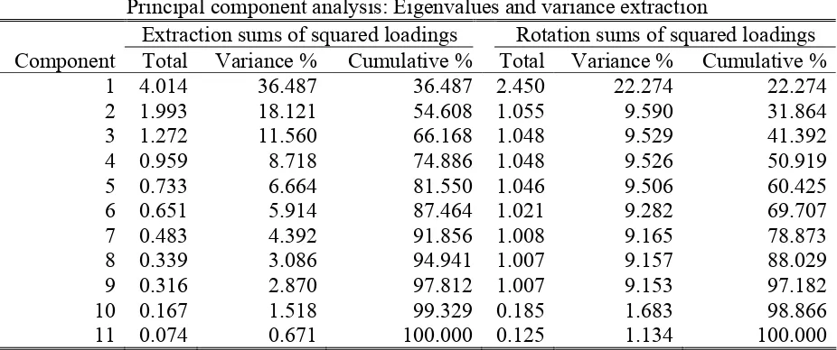
Our approach, on the contrary, is inferential and it emphasises model testing and evaluation. Initially, we perform exploratory analysis but in subsequent stages of data analysis we formally test the insights gained from the exploratory analysis. For this purpose we first perform principal component factor analysis and then test each implied dimension (factor) for specification using maximum likelihood confirmatory factor analysis. Finally, we develop a recursive structural equation model with latent variables that includes more complex relationships among the analysed variables.

3.2. Factor analysis

Table 4

Principal component analysis: Eigenvalues and variance extraction

Extraction sums of squared loadings Rotation sums of squared loadings Component Total Variance % Cumulative % Total Variance % Cumulative %

1 4.014 36.487 36.487 2.450 22.274 22.274

2 1.993 18.121 54.608 1.055 9.590 31.864

3 1.272 11.560 66.168 1.048 9.529 41.392

4 0.959 8.718 74.886 1.048 9.526 50.919

5 0.733 6.664 81.550 1.046 9.506 60.425

6 0.651 5.914 87.464 1.021 9.282 69.707

7 0.483 4.392 91.856 1.008 9.165 78.873

8 0.339 3.086 94.941 1.007 9.157 88.029

9 0.316 2.870 97.812 1.007 9.153 97.182

10 0.167 1.518 99.329 0.185 1.683 98.866

11 0.074 0.671 100.000 0.125 1.134 100.000

Keeping also in mind that we conjectured about three dimensions, i.e., factors (economic, structural and demographic) we computed factor analysis retaining three factors.

Component Number

11 10 9 8 7 6 5 4 3 2 1

Eigenv

alue

5 4

3 2

1 0

Figure 2. Cattell’s scree test

In addition, on the basis of principal component solution and insignificant correlations with other variables we dropped DISTANCE variable from further analysis. Un-rotated and rotated loadings (for the remaining ten variables) are shown in Table 5.

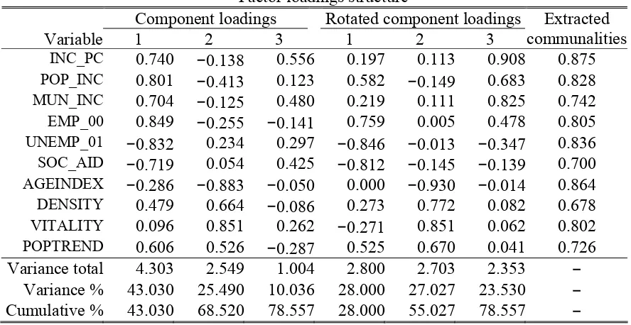
Table 5

Factor loadings structure

Component loadings Rotated component loadings

Variable 1 2 3 1 2 3

Extracted communalities

INC_PC 0.740 −0.138 0.556 0.197 0.113 0.908 0.875

POP_INC 0.801 −0.413 0.123 0.582 −0.149 0.683 0.828

MUN_INC 0.704 −0.125 0.480 0.219 0.111 0.825 0.742

EMP_00 0.849 −0.255 −0.141 0.759 0.005 0.478 0.805

UNEMP_01 −_0.832 0.234 0.297 −0.846 −0.013 −0.347 0.836

SOC_AID −_0.719 0.054 0.425 −0.812 −0.145 −0.139 0.700

AGEINDEX −_0.286 −_0.883 −_0.050 0.000 −0.930 −0.014 0.864

DENSITY 0.479 0.664 −0.086 0.273 0.772 0.082 0.678

VITALITY 0.096 0.851 0.262 −0.271 0.851 0.062 0.802

POPTREND 0.606 0.526 −0.287 0.525 0.670 0.041 0.726

Variance total 4.303 2.549 1.004 2.800 2.703 2.353 − Variance % 43.030 25.490 10.036 28.000 27.027 23.530 − Cumulative % 43.030 68.520 78.557 28.000 55.027 78.557 −

The demographic dimension (AGEINDEX, DENSITY and VITALITY) seem well captured

with the second factor. The third factor then appears to account for the economic dimension and includes INC_POP, POP_INC and MUN_INC with high loadings. However, EMP_00 appears to also load on this factor. The general impression from this three-factor solution is that there does not appear to be a “simple structure” in the data. There are several complex loadings, i.e., several variables appear to be indicators of more then one latent variable. Also, on theoretical grounds it is highly unlikely that these three underlying dimensions are uncorrelated in the population thus the above factor solution can, at best, serve as a starting point for more detailed analysis in which these indicative and partly ambiguous findings could be statistically tested.

3.3. Confirmatory maximum likelihood factor analysis

Formal testing of factor structures is most conveniently done in the confirmatory factor analysis framework using the maximum likelihood technique. Although all of our variables are continuous we have found that they are not normally distributed. Normality is, however, important in maximum likelihood estimation based on multivariate normal likelihood. We proceed by transforming the variables closer to the Gaussian distribution and this way try to avoid potential problems with the analysis of non-normal variables (see Babakus, et al., 1987; Curran, et al., 1996; West, et al., 1995). For this purpose we apply the normal scores

follows. Given a sample of N observations on the jth variable, xj= {xj1, xj2, …, xjN}, the normal scores transformation is computed in the following way. First define a vector of k distinct sample values, xjk = {xj1', xj2', …, xjk'} where k ≤ N thus xk ⊆ x. Let fi be the frequency of occurrence of the value xji in xj so that fji ≥ 1 and. Then normal scores xjiNS are computed as

xjiNS = (N/fji){φ(α j,i-1) - φ(αji)} where φ is the standard Gaussian density function, α is defined as

(

)

1 ,..., 2 , 1

0

,

, ,

1 1 1

k i

k i

i

f

N i

t jt ji

=

− =

=

    

∞ Φ

∞ −

= − −

∑

₌

α ,

and Φ-1 is the inverse of the standard Gaussian distribution function. The normal scores are further scaled to have the same mean and variance as the original variables.

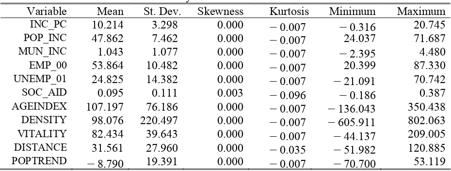
The transformation of the variables resulted in insignificant normality chi-square statistics. The mean and variances remained unaltered, though some values became negative (note the minimums) due to rescaling (Table 6).

Table 6

Univariate Summary Statistics for Continuous Variables

Variable Mean St. Dev. Skewness Kurtosis Minimum Maximum

INC_PC 10.214 3.298 0.000 -_0.007 -_0.316 20.745

POP_INC 47.862 7.462 0.000 -_0.007 24.037 71.687

MUN_INC 1.043 1.077 0.000 -_0.007 -_2.395 4.480

EMP_00 53.864 10.482 0.000 -_0.007 20.399 87.330

UNEMP_01 24.825 14.382 0.000 -_0.007 -_21.091 70.742

SOC_AID 0.095 0.111 0.003 -_0.096 -_0.186 0.387

AGEINDEX 107.197 76.186 0.000 -_0.007 -_136.043 350.438

DENSITY 98.076 220.497 0.000 -_0.007 -_605.911 802.063

VITALITY 82.434 39.643 0.000 -_0.007 -_44.137 209.005

DISTANCE 31.561 27.960 0.000 -_0.035 -_51.982 120.885

POPTREND -_8.790 19.391 0.000 -_0.007 -_70.700 53.119

0 10 20 .05

.1

INC _ PC N(s=3 .3 )

25 50 75

.02 .04

.06 POP_ INC N(s=7 .4 6 )

-2.5 0 2.5 5

.1 .2 .3

.4 MUN_ INC N(s=1 .0 8 )

25 50 75 100

.01 .02 .03

.04 EMP_ 0 0 N(s=1 0 .5 )

0 50

.01 .02 .03

UNEMP_ 0 1 N(s=1 4 .4 )

-.25 0 .25 .5

2

4 SOC _ AID N(s=0 .1 1 1 )

0 250

.002 .004

.006 AGEINDEX N(s=7 6 .1 )

-500 0 500 1000

.0005 .001 .0015

.002 DENSITY N(s=2 2 0 )

0 100 200

.005 .01

VITALITY N(s=3 9 .6 )

0 100

.005 .01

.015 DISTANC E N(s=2 7 .9 )

-50 0 50

.01 .02

POPTR END N(s=1 9 .4 )

Figure 3. Empirical density (Gaussian kernel estimate): normalised data

Table 7

Test of Univariate Normality for Continuous Variables: Normalised data

Skewness Kurtosis Skewness and Kurtosis

Variable Z-Score P-Value Z-Score P-Value Chi-Square P-Value

INC_PC 0.000 1.000 0.065 0.948 0.004 0.998

POP_INC 0.000 1.000 0.065 0.948 0.004 0.998

MUN_INC 0.000 1.000 0.065 0.948 0.004 0.998

EMP_00 0.000 1.000 0.065 0.948 0.004 0.998

UNEMP_01 0.000 1.000 0.065 0.948 0.004 0.998

SOC_AID 0.030 0.976 -_0.388 0.698 0.151 0.927

AGEINDEX 0.000 1.000 0.065 0.948 0.004 0.998

DENSITY 0.000 1.000 0.065 0.948 0.004 0.998

VITALITY 0.000 1.000 0.065 0.948 0.004 0.998

DISTANCE -_0.004 0.997 -_0.074 0.941 0.005 0.997

POPTREND 0.000 1.000 0.065 0.948 0.004 0.998

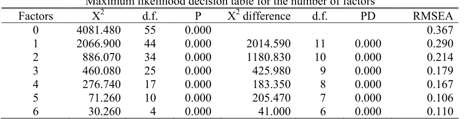
Table 8

Maximum likelihood decision table for the number of factors

Factors X2 d.f. P X2 difference d.f. PD RMSEA

0 4081.480 55 0.000 0.367

1 2066.900 44 0.000 2014.590 11 0.000 0.290

2 886.070 34 0.000 1180.830 10 0.000 0.214

3 460.080 25 0.000 425.980 9 0.000 0.179

4 276.740 17 0.000 183.350 8 0.000 0.167

5 71.260 10 0.000 205.470 7 0.000 0.106

6 30.260 4 0.000 41.000 6 0.000 0.110

RMSEA = root mean square error of approximation

In the following analysis we test separate measurement models for three implied dimensions starting from the indicative factor analysis results. Our purpose here is to statistically evaluate validity of single dimensions separately.

The confirmatory measurement models as well as later structural models are estimated within the class of general linear structural equation models (Jöreskog, 1973; Hayduk, 1987; Bollen, 1989; Hayduk, 1996; Jöreskog, et al., 2000). Denoting the latent endogenous variables by and latent exogenous variables by ξ and their respective observed indicators by

y and x, the structural part of the model is given by

(1) = B + Гξ +

The measurement models are given in form of standard factor analytic models as (2) y = Λy + є,

for latent endogenous and

(3) x = Λxξ + ,

for latent exogenous variables. Using Jöreskog’s LISREL notation we also define the following second moment matrices: E(ξξT) = Φ, E( T) = Ψ, E(єєT) = Θ_є, E( T) = Θ_δ, and

E(є T) = Θ_δє. The covariance matrix implied by the model is comprised from three separate covariance matrices, covariance matrix of the observed indicators of the latent endogenous variables

(4) Σyy = E(yyT)

= E[(Λy + є)(Λy + є)T] = ΛyE(

T

)ΛyT + Θє

the covariances between the indicators of latent endogenous and indicators of latent exogenous variables

(5) Σyx = E(yxT)

= E[(Λy + є)(Λxξ + )T] = ΛyE( ξT)ΛxT + ΘδєT

=Λy(I−B)-1ΓΦΛxT + ΘδєT,

and finally, the covariance matrix of the indicators of the latent exogenous variables (6) Σxx = E(xxT)

= E[(Λxξ + )(Λxξ + )T] = ΛxE(ξξT)ΛxT + Θδ = ΛxΦΛxT + Θδ.

Arranging the above three matrices together (noting that the lower left block is just a transpose of the upper right block we get the joint covariance matrix implied by the model, i.e.,

(7)













=

xx xy

yx yy

Σ

Σ

Σ

Σ

Σ

.

Using Eq. 4-7 the implied covariance matrix can be written in terms of model parameters as

(8) _

  

  

+ +

−

+ −

+ −

+ −

= − − ₋ − −

δ εδ

δε ε

Θ ΦΛ Λ Θ

Λ

B I

ΦΓ Λ

Θ ΓΦΛ

B I

Λ Θ Λ

B I

Ψ ΓΦΓ

B I

Λ

Σ _T

x x T

y T T

x

T T x y

T y T y

] ) [(

) ( ]

) )[( (

) (

1

1 1

1 1

.

The maximum likelihood estimates of the model parameters, given the model is identified, can be obtained by numerical maximisation of the multivariate Gaussian log-likelihood function

(9) F =lnΣ +tr

{ }

SΣ−1 −lnS−(p+q),

where p and q are the numbers of the observed indicators of latent endogenous and latent exogenous variables, respectively.

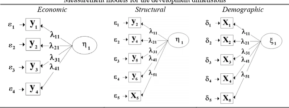
demographic). Table 9 shows conceptual path diagrams for the three hypothetical latent dimensions including complex loadings suggested from the factor solution in Table 5. Note that due to simplicity we use the LISREL notation defined in Table 1.

Table 9

Measurement models for the development dimensions

Economic Structural Demographic

The “economic” measurement model is given in matrix notation as (10) y1=Λy 1+є,

or equivalently, in terms of scalar elements of the matrices as

(11)

( )

   

 

   

 

+     

 

    

 

=    

 

   

 

4 3 2 1

1

) ( 41

) ( 31

) ( 21

) ( 11

4 3 2 1

ε ε ε ε η

λ λ λ λ

y y y y

y y y y

.

(12)               = Θ ) ( 44 ) ( 42 ) ( 33 ) ( 22 ) ( 11 0 0 0 0 0 ε ε ε ε ε ε

θ

θ

θ

θ

θ

.

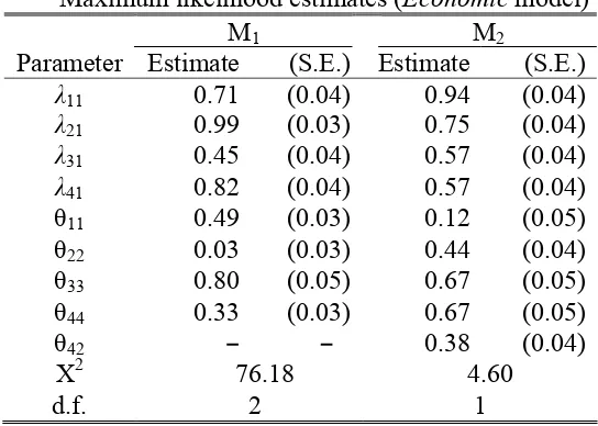
The estimation results are shown in Table 10. It can be seen that the chi-square dropped to 4.6 with 1 degree of freedom, which is no longer significant, thus the modified model M2 now fits the data.

Table 10

Maximum likelihood estimates (Economic model)

M1 M2

Parameter Estimate (S.E.) Estimate (S.E.)

λ11 0.71 (0.04) 0.94 (0.04)

λ21 0.99 (0.03) 0.75 (0.04)

λ31 0.45 (0.04) 0.57 (0.04)

λ41 0.82 (0.04) 0.57 (0.04)

θ11 0.49 (0.03) 0.12 (0.05)

θ22 0.03 (0.03) 0.44 (0.04)

θ33 0.80 (0.05) 0.67 (0.05)

θ44 0.33 (0.03) 0.67 (0.05)

θ42 − − 0.38 (0.04)

X2 76.18 4.60

d.f. 2 1

A similar procedure is used to assess the measurement model for the second hypothesised dimension (structural). Building a measurement model with three structural indicators (y4, y5,

y6) and also including y2 and x5 which had moderate loadings on this factor in the exploratory factor analysis we get

(13) y2=Λy 2+є, or in full matrix notation

(14)

( )

The inclusion of y2 (POP_INC) makes sense from the economic point of view, while the inclusion of x5 (POPTREND) is less clear. Its inclusion was based on its moderately high loading on the structural factor (Table 5) and now it can be formally tested. Table 11 gives estimates for model M1 and M2, the later one excluding x5. Though neither model has good fit, the chi-square difference between the two models is 176.34 which strongly rejects M2 in favour of M1, that is, the inclusion of the ambiguous variable (POPTREND) into the structural factor is rejected.

Table 11

Maximum likelihood estimates (Structural model)

M1 M2 M3

Parameter Estimate (S.E.) Estimate (S.E.) Estimate (S.E.)

λ11 0.81 (0.04) 0.81 (0.04) 0.79 (0.04)

λ21 0.99 (0.03) 1.01 (0.03) 1.03 (0.03)

λ31 −0.86 (0.03) −0.84 (0.04) −0.82 (0.04) λ41 −0.49 (0.04) −0.47 (0.04) −0.47 (0.04)

λ51 0.39 (0.04) − − − −

θ11 0.34 (0.02) 0.35 (0.02) 0.38 (0.03) θ22 0.02 (0.02) −0.01 (0.02) −0.06 (0.02) θ33 0.27 (0.02) 0.29 (0.02) 0.32 (0.02) θ44 0.76 (0.05) 0.78 (0.05) 0.78 (0.05)

θ55 0.85 (0.05) − − − −

θ43 − − − − 0.22 (0.02)

X2 312.51 136.17 13.21

d.f. 5 2 1

The fit of the model, however, is still not good enough, and we again modify it on the bases of the largest modification index by freeing the (4, 3) element of the Θ_є matrix, i.e.,

(15)

     

 

     

 

= Θ

) ( 55 ) ( 44 ) ( 43

) ( 33 ) ( 22 ) ( 11

0 0 0 0

0 0

0 0 0

ε ε ε ε ε ε

ε

θ

θ

θ

θ

θ

θ

,

which results in model M3 with the chi-square of 13.21 with 1 degree of freedom indicating acceptable fit of the model.

Finally, we estimate the confirmatory model for the demographic dimension noting that this was the only “simple-structured” factor, i.e., without any ambiguous loadings. The model is specified as

where the x-ξ notation indicates that this factor is treated as exogenous. This assumption will be clarified in the context of the full LISREL model in section 3.4. Remembering that we dropped the DISTANCE variable from further analysis on the basis of its low loading in principal component analysis and insignificant correlations with other variables, we are now in position to formally test its exclusion from the demographic measurement model. The model that includes the DISTANCE variable (x4) is given as

(17)

( )

     

 

     

 

+

     

 

     

 

=

     

 

     

 

5 4 3 2 1

1

) ( 51

) ( 41

) ( 31

) ( 21

) ( 11

5 4 3 2 1

δ

δ

δ

δ

δ

ξ

λ

λ

λ

λ

λ

x x x x x

x x x x x

.

We term this model M1. Model M2 setsλ41 to zero. The estimation results are shown in Table 12. M1 has a chi-square of 189.96 with 5 degrees of freedom and M2 has a chi-square of 97.89 with 2 degrees of freedom thus the chi-square difference is 92.07 which is highly significant. Therefore, we can reject the inclusion of x4 into the model.

Table 12

Maximum likelihood estimates (Demographic model)

M1 M2 M3

Parameter Estimate (S.E.) Estimate (S.E.) Estimate (S.E.)

λ11 0.98 (0.03) 1.00 (0.03) 1.06 (0.04)

λ21 -0.65 (0.04) -0.64 (0.04) -0.59 (0.04)

λ31 -0.79 (0.04) -0.78 (0.04) -0.73 (0.04)

λ41 0.30 (0.04) - - -

-λ51 -0.57 (0.04) -0.56 (0.04) -0.53 (0.04)

θ11 0.04 (0.03) 0.00 (0.03) -0.13 (0.05)

θ22 0.57 (0.04) 0.60 (0.04) 0.65 (0.04)

θ33 0.38 (0.03) 0.39 (0.03) 0.46 (0.04)

θ44 0.91 (0.06) - - -

-θ55 0.68 (0.04) 0.69 (0.04) 0.72 (0.04)

θ52 - - - - 0.28 (0.03)

X2 189.96 97.89 5.27

d.f. 5 2 1

(18)

     

 

     

 

= Θ

) ( 55 )

( 52

) ( 44 ) ( 33 ) ( 22 ) ( 11

0 0 0

0 0 0

0 0 0

δ δ

δ δ δ δ

δ

θ

θ

θ

θ

θ

θ

.

The modified model (M3) had chi-square of 5.27 with 1 degree of freedom, which now indicates acceptably good fit.

3.4. The structural equation model

Having estimated the three measurement models separately, we now estimate a joint model that includes all three dimensions simultaneously. We conducted some preliminary confirmatory analysis, using chi-square difference approach in ML estimation of restricted and unrestricted models, to test for the significance of correlations between factors finding that these are highly significant (detailed results are omitted for brevity).

Figure 5. Conceptual path diagram for the structural model

measured by its observed indicators. Furthermore we conjecture that the structural dimension is causally affected by the demographic factor. In terms of model types, this would be a linear recursive (we assume unidirectional causality) structural equation model with latent variables. Putting it all together we arrive at the model shown in Fig. 5.

Note that due to consistency with the notation defined in Table 1 we keep the symbol x5 for the POPTREND variable and drop x4 (DISTANCE) from the model. Also, on the basis of the above estimated separate measurement (factor) models and modification indices from preliminary estimation we add the suggested error covariance and complex loadings, but now we put the three measurement models together and add structural relationships among the three latent variables. In matrix notation the endogenous measurement model corresponding to path diagram shown in Fig. 5. is given by

(22)                     +                           =                     6 5 4 3 2 1 2 1 ) ( 62 ) ( 52 ) ( 42 ) ( 41 ) ( 31 ) ( 22 ) ( 21 ) ( 11 6 5 4 3 2 1 0 0 0 0

ε

ε

ε

ε

ε

ε

η

η

λ

λ

λ

λ

λ

λ

λ

λ

y y y y y y y y y y y y y y .

Similarly, the exogenous measurement model is given by

(23)

( )

            +               =             4 3 2 1 1 ) ( 41 ) ( 31 ) ( 21 ) ( 11 5 3 2 1

δ

δ

δ

δ

ξ

λ

λ

λ

λ

x x x x x x x x .

Finally, the structural part of the model is specified as follows

(24)

( )

_

     +       +             =       2 1 1 21 11 2 1 12 2 1 0 0 0 ζ ζ ξ γ γ η η β η η ,

(25)                     = Θ ) ( 66 ) ( 65 ) ( 55 ) ( 44 ) ( 33 ) ( 31 ) ( 22 ) ( 11 0 0 0 0 0 0 0 0 0 0 0 0 0 ε ε ε ε ε ε ε ε ε θ θ θ θ θ θ θ θ ,

(for the y-measurement model) and as

(26)               = Θ ) ( 44 ) ( 42 ) ( 33 ) ( 32 ) ( 22 ) ( 11 0 0 0 0 δ δ δ δ δ δ δ θ θ θ θ θ θ ,

for the x-measurement model. The parameter estimates are shown in Table 6 and Table 7. The model chi-square (normal-theory weighted) is 209.41 with 26 degrees of freedom which is appears not well fitting.

Table 6

Maximum likelihood estimates of the coefficient matrices

                  − = ) 04 (. 49 . 0 ) 04 (. 83 . 0 ) 05 (. 53 . ) 03 (. 23 . 0 ) 03 (. 23 . ) 14 (. 34 . ) 06 (. 86 . 0 ) 04 (. 41 . y Λ             − − − = (.04) 60 . (.04) 48 . (.05) 12 . (.04) .90 y Λ       − = 0 0 ) 14 (. 20 . 1 0 B _      = ) 06 (. 53 . ) 07 (. 45 . Γ

The model modification indices suggested a number of ways to modify the model. A generalisation of the model that would allow correlations between the uniquenesses of the y

and x indicators requires estimation of the Θ_δє matrix (see in particular Gerbing and Anderson, 1984).

(27)               = Θ ) ( 45 ) ( 42 ) ( 34 ) ( 32 ) ( 15 0 0 0 0 0 0 0 0 0 0 0 0 0 0 0 δε δε δε δε δε δε θ θ θ θ θ . Table 7

Maximum likelihood estimates of the error covariances

                    − = Θ ) 05 (. 70 . ) 03 (. 01 . 0 0 0 0 ) 04 (. 12 . 0 0 0 0 ) 03 (. 20 . 0 0 0 ) 05 (. 87 . 0 ) 03 (. 29 . ) 09 (. 22 . 0 ) 04 (. 59 . ε             = Θ ) 05 (. 64 . 0 ) 04 (. 08 . 0 ) 05 (. 77 . ) 04 (. 15 . 0 ) 06 (. 98 . 0 ) 05 (. 19 . δ

The estimation of the modified model (Table 8) produced very similar results to the previous model.

Table 8

Maximum likelihood estimates of the coefficient matrices (modified model)

The chi-square of the overall fit has dropped to 27.66 with 21 degrees of freedom which is insignificant (p-value = 0.15). Thus we conclude, on statistical grounds, that the estimated model has acceptable fit. Note that now an additional matrix (Θδє) is estimated (see Table 9).

Table 9

Maximum likelihood estimates of the error covariances (modified model)

                    − = Θ ) 05 (. 78 . ) 02 (. 08 . 0 0 0 0 ) 04 (. 14 . 0 0 0 0 ) 03 (. 19 . 0 0 0 ) 05 (. 86 . 0 ) 03 (. 31 . ) 09 (. 26 . 0 ) 04 (. 59 . ε             = Θ ) 05 (. 57 . 0 ) 04 (. 08 . 0 ) 05 (. 75 . ) 04 (. 15 . 0 ) 06 (. 99 . 0 ) 05 (. 32 . δ             − − = Θ ) 04 (. 29 . 0 0 ) 02 (. 11 . 0 0 ) 02 (. 11 . 0 ) 02 (. 07 . 0 0 0 0 0 0 ) 03 (. 30 . 0 0 0 0 δε

4. Estimation of latent regional development score

Using the parameters of the estimated LISREL model (Tables 8 and 9) we compute scores for the latent variables following the approach of Jöreskog, 2000. Such methods also allow structural recursive and simultaneous relationships among latent variables. Estimation of factor scores in the pure measurement (factor) models is just a special case of the general procedure (see Lawley and Maxwell, 1971).

We describe a technique capable of computing scores of the latent variables based on the maximum likelihood solution of the Eqs. (1-3) following Jöreskog (2000). Writing Eqs. (2) and (3) in a system

(28) _

and using the following notation

(29) _

     ≡       ≡       ≡       ≡ x y x ξ ξ Λ 0 0 Λ Λ x y a a , ,

, _a ,

the latent scores for the latent variables in the model can be computed using the formula (30) ξa UD1/2VL1/2VTD1/2UTΛTΘ_a x_a

1

− −

= ,

where UDUT is the singular varlue decomposition of Φa = E(ξaξaT), and VLVT is the singular value decomposition of the matrix D1/2UTBUD1/2, while Θa is the error covariance matrix of the observed variables. Derivation of the Eq. (30) follows the approach of Jöreskog (2000) and Lawley and Maxwell (1971). The latent scores ξai can be computed for each observation

xij in the (10 × N) sample matrix whose rows are observations on each of our 10 observed variables and N = 545, i.e.,

(31)                     N N N N N x x x x x x x x x x x x x x x , 10 2 , 10 1 , 10 4 42 41 3 32 31 2 22 21 1 12 11 L M L M M L L L L

= (x1x2⋅⋅⋅xN).

Having computed the latent scores for

η1

,

η2

and

ξ1

we can use the information from the model to rank and compare development level for all territorial units. The model in Fig. 5 implies an underlying economic development level that is simultaneously determined by the structural and demographic factors and measured by several observed indicators. It is clear that such model, in principle, extracts far more information about the development level then using a single observed indicator of latent economic development such as the GDP per capita (the EU methodology for Structural Funds allocation). With latent scores it is now possible to estimate a simple linear equation (using OLS) with

η1

as endogenous variable. This produces the following result

) 006 . 0 ( ) 033 . 0 ( ) 291 . 2 ( 087 . 0 102 . 1 170 .

74 _{1 2}

1

ξ

η

η

= − +

with R2 = 0.825 and the Wald test of 1281.7 which indicates very good fit and well determined coefficients. What the above equation suggests is that

η1

is a linear function of

η2

and

ξ1

and thus the territorial units can be ranked either on the grounds of

η1

or by −.102ξ1 + .087η2 (ignoring the constant). Using 100 least developed municipalities (18%) ranked on the bases of −.102ξ1 + .087η2 and η1 we can compare how many of them entered the first 100 in each of the two cases. The cross-tabulations in Table 10 shows that 70 municipalities were ranked within 100 least developed by both methods (about 13%). The most likely funding allocation given constraints to the national budget will include 5-10% of least developed municipalities, thus this type of summary statistics shows a clear comparative picture regarding classification and ranking performance of the alternative criteria.

Table 10 Crosstabulation count

Criteria −.102ξ1 + .087η2 η1

Group < 100 > 100 Total −.102ξ1 + .087η2 < 100 70 29 99

η1 > 100 29 417 446

Total 99 446 545

Similarly, we can use latent scores from alternative models and subsequently cross-tabulate the results checking how many units enter some predefined cut-off criteria such as least developed group of municipalities.

5. Conclusion

development level, and (iii) selection of a given percentage of units for inclusion into a national subsidy programme.

Acknowledgments

We wish to acknowledge the support of the Ministry for Public Works, Reconstruction and Construction of the Republic of Croatia in carrying out the project “Criteria for the Development Level Assessment of the Areas Lagging in Development” which served as the basis for this paper. We wish to thank the University of Zagreb, the Croatian Health Insurance Institute, Ministry of Finance, Ministry of Justice, Administration and Local Government, Ministry of the Interior and the Croatian Employment Office for valuable help in data collection.

References

Anderson, T.W. (1984), “An Introduction to Multivariate Statistical Analysis”, New York: John Wiley.

Babakus, E., Ferguson, C.E., Jr., and Joreskog, K.G. (1987), “The sensitivity of confirmatory maximum likelihood factor analysis to violations of measurement scale and distributional assumptions”, Journal of Marketing Research, 24, pp. 222-28.

Bai, J. and Ng, S. (2002), “Determining the Number of Factors in Approximate Factor Models”, Econometrica, 70, pp. 191-221.

Blasius, J. and Greenacre, M. (1998), Visualization of Categorical Data. Academic Press. Bollen, K.A. (1989), Structural Equations with Latent Variables. New York: Wiley.

Bollen, K.A. (2001), “Modeling Strategies: In Search of the Holy Grail”, Structural Equation

Modeling, 7, pp. 74-81.

Borg, I. And Groenen, P. (1997), Modern Multidimensional Scaling. Berlin: Springer.

Bowman, K.O. and Shenton, L.R. (1975), “Omnibus Test Contours for Departures from Normality based on √b1 and b2”, Biometrika, 62, pp. 243-50.

Buntig, B., Saris, W.E. and McCormack, J.A. (1987), “Second-order Factor Analysis of the Reliability and Validity of the 11 plus examination in Northern Ireland”, The Economic

and Social Review, 18, pp. 137-147

Curran, P.J., West, S. G., and Finch, J. F. (1996), “The robustness of test statistics to nonnormality and specification error in confirmatory factor analysis”, Psychological

Methods, 1, pp. 16-29.

Belanger, A. and D’Agostino, R. B. (1990), “A suggestion for using powerful and informative tests of normality”, American Statistician, 44, pp. 316-321.

D’Agostino, R.B. (1970), “Transformation to Normality of the Null Distribution of g1”,

Biometrika, 57, pp. 679-681.

D’Agostino, R.B. (1971), “An Omnibus Test of Normality for Moderate and Large Sample Size”, Biometrika, 58, pp. 341-348.

D’Agostino, R.B. (1986), “Tests for Normal Distribution”, in D’Agostino, R.B. and Stephens, M.A. (Eds.), Goodness-of-fit Techniques. New York: Marcel Dekker, pp. 367-419. Doornik, J.A., and Hansen, H. (1994), A Practical Test for Univariate and Multivariate

Normality, Discussion paper, Nuffield College, Oxford.

Everitt, B.S. (1993), Cluster Analysis. New York: John Wiley.

Gerbing, D.W. and Anderson, J.C. (1984), “On the Meaning of Within-factor Correlated Measurement Errors”, Journal of Consumer Research, 11, pp. 572-580.

Gerbing, D.W., Hamilton, J.G. and Freeman, E.B. (1994), “A Large-scale Second-order Structural Equation Model of the Influence of Management Participation on Organizational Planning Benefits”, Journal of Management, 20, pp. 859-885.

Greenacre, M. (1993), Correspondence Analysis in Practice. Academic Press.

Greenacre, M. and Blasius. J., ed. (1994), Correspondence Analysis in the Social Sciences:

Recent Developments and Applications. Academic Press.

Hayduk, L. (1987), Structural Equation Modeling with LISREL. Baltimore: John Hopkins University Press.

Hayduk, L. (1996), LISREL: Issues, Debates and Strategies. Baltimore: John Hopkins University Press.

Hendry, D.F. and Doornik, J.A. (1999), Empirical Econometric Modelling Using PcGive, Vol. I. West Wickham: Timberlake Consultants.

Jöreskog, K.G. (1973), “A General Method for Estimating a Linear Structural Equation System”, in Goldberger, A.S. and Duncan, O.D. (Eds.), Structural Equation Models in

the Social Sciences. New York: Seminar Press.

Jöreskog, K.G. (1999), “Formulas for skewness and kurtosis”, Scientific Software International, http://www.ssicentral.com/lisrel.

Jöreskog, K.G. (2000), “Latent variable scores and their uses”. Scientific Software International, http://www.ssicentral.com/lisrel.

Jöreskog, K.G., Sörbom, D. du Toit, S. and du Toit, M. (2000), LISREL 8: New Statistical

Features. Chicago: Scientific Software International.

Jöreskog, K.G. and Sörbom, D. (2001), LISREL 8: New Statistical Features. Chicago: Scientific Software International.

Kaplan, D. and Elliott, P.R. (1997a), “A Model-based Approach to Validating Educational Indicators using Multilevel Structural Equation Modeling”, Journal of Educational and

Behavioral Statistics, 22, pp. 232-348.

Kaplan, D. and Elliott, P.R. (1997b), “A Didactic Example of Multilevel Structural Equation Modeling Applicable to the Study of Organizations”, Structural Equation Modeling, 4, pp. 1-24.

Lawley, D.N. and Maxwell, A.E. (1971), Factor Analysis as a Statistical Method. 2nd ed. London: Butterworths.

Lipshitz, G. and Raveh, A. (1994), “Application of the Co-plot method in the study of socio-economic differences among cities: a basis for a differential development policy”,

Urban Studies, 31, pp. 123-135.

Lipshitz, G. and Raveh, A. (1998), “Socio-economic Differences among Localities: A New Method of Multivariate Analysis”, Regional Studies, 32, pp. 747-757.

Maleković, S. (2001), Criteria for the Development Level Assessment of the Areas Lagging in

the Development. Zagreb: IMO.

Mardia, K.V. (1980), “Tests of Univariate and Multivariate Normality”, in Krishnaiah, P.R. (Ed.), Handbook of Statistics, Vol. I. Amsterdam: North Holland, pp. 279-320.

Mulaik, S.A. (1972), The Foundation of Factor Analysis. New York: McGraw-Hill.

Mulaik, S.A. and Quartetti, D.A. (1997), “First Order or Second Order General Factor?”,

Structural Equation Modeling, 4, pp.193-211.

Shenton, L.R. and Bowman, K.O. (1977), “A Bivariate Model for the Distribution of √b1 and b2”, Journal of the American Statistical Association, 72, pp. 206-211.

Tacq, J. (1998), Multivariate Analysis Techniques in Social Science Research. London: Sage. Weller, S.C. and Romney, A.K. (1990), Metric Scaling: Correspondence Analysis. London:

Sage.

West, S. G., Finch, J.F. and Curran, P.J. (1995), “Structural equation models with nonnormal variables: Problems and remedies”, in Hoyle R.H. (Ed.), Structural Equation Modeling: