Factors Determination that Influence Food Insecurity in Central Java Using Spatial Panel Data Analysis

(1)

FACTORS DETERMINATION THAT INFLUENCE FOOD INSECURITY

IN CENTRAL JAVA USING SPATIAL PANEL DATA ANALYSIS

LIA RATIH KUSUMA DEWI

DEPARTMENT OF STATISTICS

FACULTY OF MATHEMATICS AND NATURAL SCIENCES BOGOR AGRICULTURAL UNIVERSITY

(2)

ABSTRACT

LIA RATIH KUSUMA DEWI. Factors Determination that Influence Food Insecurity in Central

Java Using Spatial Panel Data Analysis. Advised by ASEP SAEFUDDIN dan YENNI

ANGRAINI.

Food insecurity refers to the consequence of inadequate consumption of nutritious food at region, society or household, considering the physiological use of food by the body as being within the domain of nutrition and health. Sutawi (2008) explained that availability and achievability on aggregate scale, Indonesia citizen is appertained food secure. However, household with food insecure still found in almost whole provinces with high proportion. So, it is necessary to do a research to determine factors that influence food insecurity in a province by calculating spatial effect of inter-regency or municipality. In this research, food insecurity that will be analyzed is food insecurity in Central Java using spatial panel data analysis. Cross-section unit in this research is 35 regencies or municipalities in Central Java province which was observed for 4 years (2007-2010) as time series unit.The analysis result in this research show that fixed effect model with SAR are better used for modelling food insecuity in Central Java. This model show that production of paddy (X2) and local government original receipt of regency or municipality (X3) influence percentage of citizen with food insecure that consume calorie under basic requirement 2100 kkal/capita/day (Y) with R2 95.88%. Coefficient of λ indicates that spatial autoregressive effect significant in influencing percentage of citizen with food insecure in Central Java.

.

(3)

FACTORS DETERMINATION THAT INFLUENCE FOOD INSECURITY

IN CENTRAL JAVA USING SPATIAL PANEL DATA ANALYSIS

LIA RATIH KUSUMA DEWI

Minithesis

to complete the requirement for graduation of Bachelor Degree in Statistics

at Department of Statistics

DEPARTMENT OF STATISTICS

FACULTY OF MATHEMATICS AND NATURAL SCIENCES BOGOR AGRICULTURAL UNIVERSITY

(4)

Title : Factors Determination that Influence Food Insecurity in Central Java Using Spatial Panel Data Analysis

Name : Lia Ratih Kusuma Dewi

NRP : G14080043

Approved by

Advisor I, Advisor II,

Dr. Ir. Asep Saefuddin, M.Sc Yenni Angraini, S.Si, M.Si

NIP. 195703161981031004 NIP. 197805112007012001

Acknowledged by: Head of Department of Statistics Faculty of Mathematics and Natural Sciences

Bogor Agricultural University

Dr. Ir. Hari Wijayanto, M.Si NIP. 196504211990021001

(5)

ACKNOWLEDGEMENTS

The author felt deeply grateful Alhamdulillah to Allah SWT for deliverancing and blessing.

Especially in completing this minithesis with title “Factors Determination That Influence Food

Insecurity in Central Java Using Spatial Panel Data Analysis” as the requirement for graduation of Bachelor Degree in Statistics at Department of Statistics, Faculty of Mathematics and Natural Sciences, Bogor Agricultural University.

I recognized that the completion of this minithesis would not be done without invaluable help from other people. I am very appreciating and really thank you for their helps, ideas, critics, advices and improvement my minithesis started from begining during the progress until it was done. Therefore, I would like to express my graceful to:

1. Dr. Ir. Asep Saefuddin, M.Sc, Yenni Angraini, S.Si, M.Si, and Dr. Anang Kurnia for their great advice, support, knowledge and patience while finished this research.

2. All the lectures, administration, and library staffs in Department of Statistics, who had patiently taught and served very well.

3. POM, Karya Salemba Empat, and P.T Perfetti Van Melle for schoolarships that had been given

and could help me on finished my study.

4. My beloved parents Sugiyat and Teliah, S.Pd, my lovely brothers , Deni Wahyu Kusuma Jati,

and Aziz Kusuma Wardana, who never stopped supporting, advising, and praying for me until the end of my study.

5. Diah Kartika Pratiwi, my beloved same age cousin, for your cheering up and Rodli Abdul Latif, my adviser, for your advised, supported and cheered up my life, thanks for everything that you have done during this seven years.

6. All my friends in “Statistics 45th”, especially for “Empat Sekawan” Gusti Andhika P, Umi Nur

Chasanah, Nur Hikmah, and Astri Fitriani, thank you for our beautiful friendship and also for Yulia Anggraeni, Nur Syita P, Ramadiyan F, Didin S who had always helped and supported me to finished this minithesis.

7. My beloved family in Bogor, “Winning Eleven” (Ubi, Ompu, Choi Young Be, Mba Shin, Desseh, Mba Na, Idun, Bang Ros, Iza and Etica), Juli S, and all member of Wisma Kompeten for our great friendship, understood, supported and happiness.

8. Kak Mo, Kak Achi, Hairul, Ermi and all family of Kopma IPB for our great

“UσSHAKEABLE!” experiences.

Hopefully, this research can be useful and able to improved in the future.

Bogor, December 2012

(6)

BIOGRAPHY

Lia Ratih Kusuma Dewi was born in Klaten on November 21st 1990 as the middle daughter of

Sugiyat and Teliah, S.Pd from three siblings, Deni Wahyu Kusuma Jati and Aziz Kusuma Wardana. She finished her education from SD N 1 Jurang Jero at 2002 and graduated from SMP N 1 Karanganom at 2005. She graduated her senior high school at SMA N 1 Karanganom at 2008 and she continued her study in Bogor Agricultural University through USMI and took Statistics as her major in Department of Statistics and choose Economics and Development Study in Department of Economics as her minor.

During learning, the author actived in several organizations, such as Koperasi Mahasiswa IPB as staff of administration, financial and personnel (2008-2011) then as director of administration, financial and personnel (2011-2012) and Profession Union Gamma Sigma Beta as secretary (2011). Other than organization, she also actived in several committees, such as Welcome Ceremony of Statistics as secretary (2011), G-Force 46 as secretary (2010), The 6th Statistika Ria (2010) as public relations, Pesta Sains 2009 as secretary, The 5th Statistika Ria (2009) as secretary, MPKMB 46 (2009) as secretary, and TPB Cup as terasurer (2009). Beside in organization and committes, she also filled her free time to be lecturer assistant (Statistical Methods (2011 & 2012), Regression Analysis (2011), and Analysis of Categorical Data (2012)), Consultant of Statistics in Expert (2010), and staff of lecturer in MSCollage Course (2010-2012) for Basic of Mathematics, Calculus and Statistical Methods .The author did intership at February

13rd until April 6th 2012 in Balai Besar Oraganisme Pengganggu Tumbuhan (BBOPT) Karawang,

(7)

LIST OF TABLE

Page

Table 1 The result of pooled model ... 5

Table 2 The result of fixed effect model ... 5

Table 3 The result of random effect model ... 5

Table 4 The result of LM-Test... 6

Table 5 Estimation and examination parameter of SAR model ... 6

Table 6 The result of Glejser test for SAR ... 7

Table 7 The result of multicollinearity test for SAR ... 7

LIST OF FIGURE

Page Figure 1 Probability plot of residual ... 7

LIST OF APPENDIX

Page Appendix 1 Description of response and explanatory variables ... 10

Appendix 2 Average value of response variable for whole regency or municipality ... 10

Appendix 3 The result of panel data analysis for pooled model ... 11

Appendix 4 The result of panel data analysis for fixed effect model ... 11

Appendix 5 The result of panel data analysis for random effect model ... 11

Appendix 6 Cross-section effect value (�_�) ... 12

(9)

1

INTRODUCTION Background

Food is the necessary basic needed for everybody through physiological, social, and antrhopological. Food always related with society effort for living on. If this primary requirement unfulfilled, then food insecurity will impact for various life aspect (Maria 2009). Food security refers to a household's physical and economic access to adequate, safe, and nutritious food that fulfills the dietary needs and food preferences of household for living an active and healthy life. Food security levels are classified into four explained that availability and achievability on

aggregate scale, Indonesia citizen is

appertained food secure. However, household with food insecure still found in almost whole provinces with high proportion. Based on National Socio-Economic Survey data of Statistics Indonesia in 2006, the lowest percentage of citizen with food insecure was at Bali province (4.8%) and the highest was at Special District of Yogyakarta (20%). Even in whole provinces which well known as central location of food production like South Sumatera, South Sulawesi, East Java, West Java, and Central Java, had high proportion of food insecure citizen over 10%.

Based on the above informations, it is necessary to do a research to determine factors that influence food insecurity in a province by calculating spatial effect of inter-regency or municipality. In this research, food insecurity that will be analyzed is food insecurity in Central Java, province with the lowest average expenditure per capita for food in Java island based on Statistics Indonesia in 2008. The data from this research is spatial panel data built by cross-section and time series data that have specific interaction between spatial units. So, the analysis that can be used for this data type is spatial panel data analysis.

Objective

The aim of this research is to determining factors that influence food insecurity in Central Java using spatial panel data analysis.

LITERATURE REVIEW Food Insecurity

Food insecurity refers to the consequence of inadequate consumption of nutritious food at region, society or household, considering the physiological use of food by the body as being within the domain of nutrition and health. Those are two form of food insecurity, first, chronic food insecurity, that can be happened repeatedly in certain of time because of low purchasing power and low quality of resource. Second, transient food insecurity is happened because of urgen situation like purchasing. This research used regression analysis. Laelati (2012) explained that food insecurity a province can be influenced by food insecurity from each regency or municipality in that province. This research result explained that factors that influence food insecurity using panel data analysis are general allocation fund, local government original receipt, income percapita, harvested area of paddy, and production of paddy.

General Model of Panel Data If the same units of observation in a cross-sectional sample are surveyed two or more times, the resulting observations are described as panel data set. Cross-section data refers to data that are collected from many units or subjects at one point in time. Time series data is a set of observations on the values that a variable takes at different times. There are another names for panel data, such as pooled data (pooling of time series and cross-sectional observations), combination of time series and

cross-section data, micropanel data,

longitudinal data (a study over time of a variable or group of subject), event history analysis and cohort analysis.

(10)

2

first by spatial units then by time (Elhorst 2010).

A panel data regression differs from a regular time-series or cross-section regression, in that it has a double subscript on its

observation and t time period. α is a scalar,β

is a vector that have measure K x 1, xit is a

where τidenotes the unobservable individual-specific effect and ɛit denotes error for i observation and t time period. (Baltagi 2005). Pooled Model

Pooled model is one of the models panel data analysis. Assumption in this model is the regression coefficient (constanta or slope) between cross-section unit and time series unit is the same. Then, to estimate the parameters independent and identically distributed IDD (0, _ε2_{), (3) E(X}

it,εit) = 0, Xit are assumed independent with εit for all i and t (Baltagi 2005).

Parameters estimation in fixed effext model is estimated by within estimator, can be explained as follows :

For the panel data regression,

y_it =α+�′_it�+τ_i+�_�� [4] these equation are averaged for over time gives:

�= �+ ��′. + τi + ��. [5]

therefore, subtracting equation [5] from [4] equation gives

individuals randomly from a large population. The assumptions for this model are (1) τi is

normal distribution (0, 2

), ) εit disturbances

stochastic independent and identically

distributed IDD (0, _ε2_{), (2) E(X}

it, τi) = 0 and

E(Xit,εit) = 0, Xit are assumed independent with εit for all i and t.

Consistent estimator obtained by OLS, but this case can make unbiased standart error. Therefore, Generalize Least Square (GLS) is better used for this model. (Baltagi 2005). Chow Test

Chow test is used for examining the significant between pooled model and fixed effect model. The hypothesis for this test is:

H0 :

τ

1 =

τ

2 = ... =

τ

N-1 = 0 (the model followed pooled model) H1 : There is one minimum i so

τ

i≠ 0 (the

model followed fixed effect model)

The test statistic for Chow test is: F₀ =(RRSS−URSS )/(N−1) regression, N denotes quantity of observations and K denotes quantity of variables. The decision for reject H0 if F0 > FN-1,N(T-1)-K,αor if p-value < α (Baltagi 2005).

Hausman Test

(11)

3

then tend to use fixed effect model. The hypothesis for this test is:

H0 : E(τi|Xit) = 0 (the model followed random effect model)

H1 : E(τi|Xit) ≠ 0 (the model followed fixed effect model)

The test statistic for Hausman test :

�hit2 =� ′[Var(� )]−1� [8] effect will have specifying interaction between spatial units. The model may contain a spatially lagged dependent variable or spatial autoregressive process in the error term, it is called spatial autoregressive model (SAR) and spatial error model (SEM) (Elhorst 2010).

SAR focus on spatial correlation of

explanatory variable, while the SEM focus on the shape of error (Anselin 2009). The structure of spatial panel data is sorted first by time and then by spatial units (Elhorst 2010). Spatial Autoregressive Model (SAR)

The spatial autoregressive model

expressed by the following equation: y_it =λ N w_ijy_jt

j=1 +�′it�+τi+εit [9]

where λ is called the spatial autoregressive coefficient and wij is an element of a spatial

weights matrix (W) describing the spatial

arrangement of the units in the sample and i≠ j. Estimation for parameters in this model using Maximum Likelihood Estimator (MLE) (Elhorst 2010).

where ϕ reflects the spatially autocorrelated

error term and ρ is called the spatial

autocorrelation coefficient. Estimation for

parameters in this model using MLE (Elhorst 2010).

Spatial Weight Matrix

Spatial weight matrix is a weight matrix summarizes the spatial reliationship in the data. The main diagonal from this matrix unit if both areas share a common edge or vertex.

After determining spatial weight matrix that will be used, then do normalization. This means that matrix is transformed so that each of the rows/collumn sums to one. It is common, but not necessary for normalization matrix is used row-normalizing.

Column-normalizing is the other method for

The examining of spatial interaction effects in cross-sectional data developed Lagrange Multiplier (LM) tests for a spatially lagged dependent variable and a spatial error correlation. The hypothesis for this test is :

a. Spatial autoregressive model

H0 : λ = 0 (there is no dependence of spatial autoregressive)

(12)

4

The test statistic for LM used: LM_λ =[�′ ��⊗ /σ 2]2

product, I_T_{denotes the identity matrix and it is} subscript the order of this matrix, � 2 denotes mean square error of panel data model, W denotes spatial weights matrix which have been normalized and e _{denotes the residual} vector of a pooled regression model without any spatial or timespecific effects or residual vector of panel data with fixed/random effect with spatial and/or time period. Finally, J and

Tware defined by : denotes the trace of a matrix. The decision for reject H0 if the value of LM statistic greater sources: National Sosio-Economic Survey, Data and Proverty Information, and Central Java in Figure. Response variable of this research is percentage of citizen with food insecure in each regency or municipality. The number of explanatory variables are five variables. Cross-section unit in this research is 35 regencies or municipalities in Central Java province which was observed for four years (2007-2010) as time series unit. Description of the variables can be seen in Appendix 1.

Method

Methodologies of this research are summarized as follows:

1. Exploration of data to observe the

characteristic of data. 2. Perform panel data analysis :

a. Estimate the parameter of pooled

d. Estimate the parameter of random effect

model.

e. Examine the significance of random

effect model or fixed effect model by using the Hausman test. If H0 is accepted, the random effect model is used, but if H0 rejected then fixed effect model is used.

3. Determine the spatial weights matrix (W).

4. Examine the effect of spatial interaction by using Lagrange Multiplier (LM) test.

5. Estimate the parameters for the equation of

spatial panel data model.

6. Examine the assumptions

RESULT AND DISCUSSION Data Exploration

Average value for over time of response variable for whole regency or municipality can be seen in Appendix 2. From this exploration is gotten information that Wonosobo is a regency with the highest average value of citizen percentage with food insecure with 27.1%. Wonosobo has the lowest total of local government original receipt and actual receipt of region when compared with another regencies with characterictic similarity of

agricultural (Kudus, Banjarnegara,

Purbalingga, and Temanggung).

(13)

5

Another information from this exploration is found some groups of regencies or municipalities that neighboring with average value of citizen precentage with food insecure almost same. The first group consist of Purbalingga, Banjarnegara, Kebumen, and Wonosobo with average value of citizen Magelang, Purworejo, and Temanggung with average value of citizen precentage with food insecure revolve 16%.

Based on that information it has possibility that food insecure could be influenced by closeness inter region or municipality. It can

be happened because of characteristic

similarity from those regencies or

municipalities.

According to the data, can be seen that percentage of citizen with food insecure that consume calorie under basic requirement 2100

kkal/capita/day (Y) and percentage of

expenditure percapita for food (X5) have high stretches of value as compared to the other variables. To solve this problem, natural logarithm transformation is taken for whole variables.

Panel Data Analysis

This research used alpha 5%. The result for estimating parameter of panel data analysis for pooled model, fixed effect model and random effect model are presented in Table 1, Table 2 and Table 3. From Table 1, explanatory variables that significant for pooled model are local government original receipt of regency or city (X3) and percentage of expenditure per capita of regency or city for food (X5) with R2 value is 41.34%.

Tabel 1 The result of pooled model

Variable Coefficient P-Value

C 1.097 0.491

government original receipt of regency or

municipality (X3). R2 value for this model is 95.13%.

Tabel 2 The result of fixed effect model

C 10.251 0.000

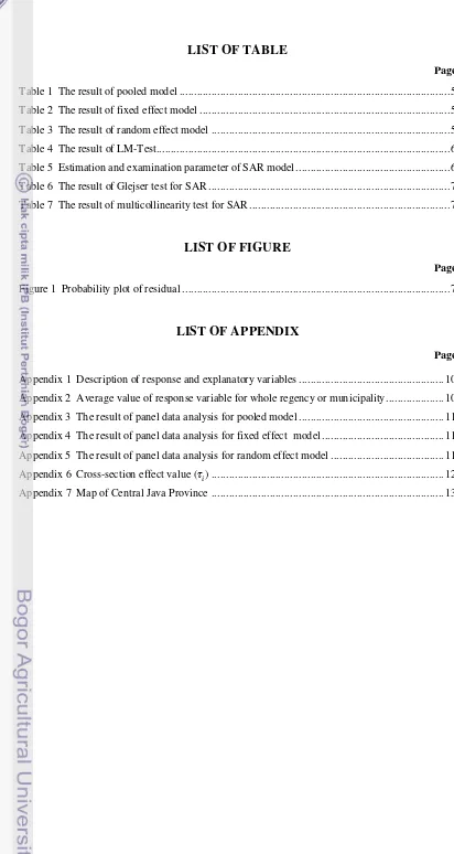
And explanatory variables that significant for random effect model are harvested area of paddy (X1), production of paddy (X2) and local government original receipt of regency or municipality (X3) that can be seen in Table 3. R2 value for this model is 95.17%.

Tabel 3 The result of random effect model

C 5.544 0.000

The complete result for estimating parameter of panel data model can be seen at model. Statistic value of cross-section F that is goten is 32.457 with value 0.000, where p-value (0.000) < alpha (0.05), so H0 is rejected. It shows that appropriate model that is used for temporary is fixed effect model. The complete result of calculation for this test can be seen at Appendix 6. Furthermore will be done Hausman Test.

Hausman Test

(14)

6 spatial effect is Lagrange Multiplier Test (Test). Before analyze spatial effect with LM-Test, it is required determination spatial weight matrix. The most natural way to represent the spatial relationships with area data is through the concept of contiguity. Contiguity concept that is used in this research is queen contiguity because this concept more reguler to used and from data exploration is estimated that food insecure could be influenced by closeness inter region or municipality. And from the map could be seen that neighborhood position be in edge (side) and corner (vertex).

After determining spatial weight matrix then next step is normalization. This means

Spatial effect can be detected by Lagrange Multiplier (LM) tests for spatial autoregressive model (SAR) and spatial error model (SEM). The calculation result can be seen in Table 4. LM-value for SAR is 63.956bigger than χ2(1) (3.841) at α =5% or p-value (0.000) < α (0.05). And LM-value for coefficient SEM is 937.211,bigger than χ2(1) (3.841) at α =5% or p-value (0.000) < α (0.05). So for both test H0 is rejected. It means that those are dependence of spatial autoregressive and spatial error. Tabel 4 The result of LM-Test

LM-Value χ2(1) P-value

SAR 63.9561 3.841 0.000

SEM 937.211 3.841 0.000

Because both tests are significant, estimate the specification is appointed by the empirical literatur. Elhorst (2010) gave example that in the empirical literatur on strategic interaction among local government, the situation where taxation and expenditures on public service interact with taxation and expenditures on public services in nearby jurisdiction is follow

theoretically consistent for the spatial

autoregressive model. And from exploration data was gotten that it has possibility that food insecure in a regency or municipality could be

influenced or have interact with regencies or municipalities nearby. So the model that will be estimates is SAR.

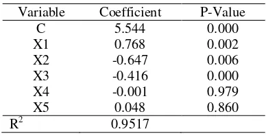
Spatial Autoregressive Model (SAR) Variables that significant in fixed effect model are production of paddy (X2) and local government original receipt of regency or municipality (X3). Two of those variables are used to build SAR model. The estimation and examine result of the parameter can be seen in Table 5. Variables production of paddy (X2), local government original receipt of regency or municipality (X3), and λ significant at α = 5%, that can be seen from p-value < α (0.05) with R2 95.88%.

Tabel 5 Estimation and examination parameter of SAR model

Variable Coefficient P-value

X2 -0.406 0.000

calorie under basic requirement 2100

kkal/capita/day (Y) in 35 regency or

The above models have cross-section effect value (�_�) that can be seen in Appendix 8. Examination The Assumption of SAR

Assumptions that must be fulfilled are residual deviation is homogenous,

non-autocorrelation inter residual, residual

normality, and no multicollinearity.

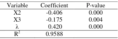
Examination the first assumption,

(15)

7

alpha 5%. It provides an explanation that homogeneity assumption is fulfilled.

Tabel 6 The result of Glejser test for SAR

C 0.4258 0.068

X2 -0.008586 0.100

X3 -0.01510 0.235

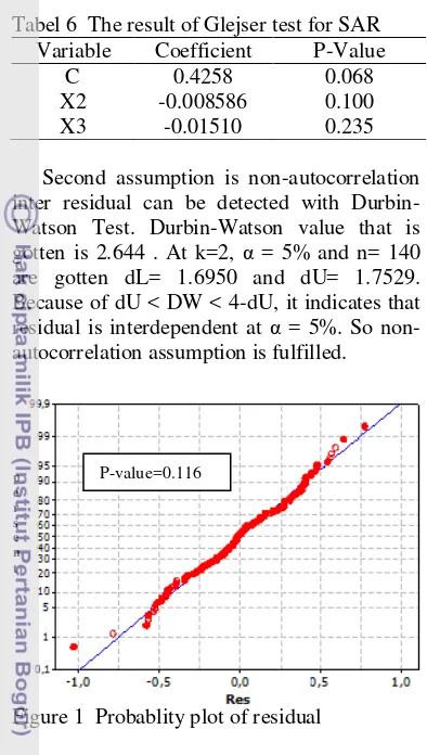
Second assumption is non-autocorrelation inter residual can be detected with Durbin-Watson Test. Durbin-Durbin-Watson value that is gotten is 2.644 . At k=2, α = 5% and n= 140

are gotten dL= 1.6950 and dU= 1.7529.

Because of dU < DW < 4-dU, it indicates that residual is interdependent at α = 5%. So non-autocorrelation assumption is fulfilled.

Figure 1 Probablity plot of residual

Third assumption is residual normality can be detected with Kolmogorov-Smirnov Test. H0 for this test is residual from model has normal distribution. P-value that is gotten is 0.116, biger than α = 5%. It indicates that

residual from this model is normal

distribution, the assumption is fulfilled. The last assumption that must fulfilled is no multicollinearty inter explanatory variables. For detecting multicollinearity, can be

detected with Variance Inflation Factors(VIF)

value. If for all explanatory variables have

VIF-value < 10, it means that no

multicollinearity inter explanatory variables. Based on Table 7, all explanatory variables have VIF-value < 10, it provides an explanation that no-multicollinaerity assumption is fulfilled.

Tabel 7 The result of multicollinearity test for SAR influence percentage of citizen with food insecure that consume calorie under basic requirement 2100 kkal/capita/day (Y) with R2 95.88%. Coefficient of λ indicates that spatial autoregressive effect significant in influencing percentage of citizen with food insecure in Central Java.

Recommendation

Based on that result, for government it is

suggested to decide foreigh for increasing

production of paddy and local government original receipt. For the next researcher, it is suggested to use another contiguity concept like distance or characteristic similarity of economic region (local government original receipt of regency, general allocation fund, etc).

REFERENCE

Anselin L. 2009. Spatial Regression.

Fotheringham AS, PA Rogerson, editor, Handbook of Spatial Analysis.London : Sage Publications.

Baltagi BH. 2005. Econometrics Analysis of Panel Data Third Edition. England : John Wiley and Sons, LTD.

Dray S et al. 2006. Spatial modeling: a comprehensive framework for principal coordinate analysis of neighbor matrices (PCNM). Ecological Modelling 196 483-493.Department of Biology, University of Regina.

Dubin R. 2009. Spatial Weights.

Fotheringham AS, PA Rogerson, editor, Handbook of Spatial Analysis. London : Sage Publications.

Elhorst JP. 2010. Spatial Panel Data Models. Fischer MM, A Getis, editor, Handbook of Applied Spatial Analysis. New York : Springer.

Food Security Council. 2006. Kebijakan

Umum Ketahanan Pangan 2006-2009.

Jakarta.

Gujarati DN. 2009. Basic Econometrics. Fifth

Edition. Singapore: The McGraw-Hill

(16)

8

Maria R, Da LS, Utma A, Simon S. 2009.

Faktor-Faktor yang Mempengaruhi

Ketersediaan Pangan Pokok Rumah

Tangga Petani di Desa Oenenu Utara Kecamatan Bikomi Tengah Kabupaten

TTU. Department of Nutritient and Society

Health. Nusa Cendana University. NTT. Nurfitriani L. 2012. Analisis Kinerja Fiskal

dan Faktor-Faktor yang Mempengaruhi Ketahanan Pangan di Provinsi NTT

[Minithesi]. Bogor: Faculty of Economics, Bogor Agricultural University.

Saliem H et al . 2001. Analisis Ketahanan Pangan Tingkat Rumah Tangga dan Regional. Research and Development Agricultural Socio-Economics Center. Bogor.

Sutawi. 2008. Tinjauan Distribusi Pangan.

(17)

9

(18)

10

Appendix 1 Description of response and explanatory variables Name of

Variables

Description Source Unit

Y Percentage of citizen with food insecure that

consume calorie under basic requirement 2100 kkal/capita/day

X2 Total number of paddy production in each regency

or municipality

Central Java in Figure

ton

X3 Total number of local government original receipt

in each regency or municipality

Central Java in

Appendix 2 Average value for over time of response variable for whole regency or municipality

Region/Municipality i. Region/Municipality i.

Cilacap 0.203 Kudus 0.108

Banyumas 0.216 Jepara 0.103

Purbalingga 0.266 Demak 0.207

Banjarnegara 0.263 Semarang 0.112

Kebumen 0.265 Temanggung 0.153

Purworejo 0.179 Kendal 0.205

Wonosobo 0.271 Batang 0.174

Magelang 0.157 Pekalongan 0.184

Boyolali 0.161 Pemalang 0.221

Klaten 0.201 Tegal 0.152

Sukoharjo 0.121 Brebes 0.252

Wonogiri 0.198 Magelang (Municipality) 0.105

Karanganyar 0.154 Surakarta (Municipality) 0.146

Sragen 0.196 Salatiga (Municipality) 0.084

Grobogan 0.203 Semarang (Municipality) 0.053

Blora 0.184 Pekalongan (Municipality) 0.087

Rembang 0.266 Tegal (Municipality) 0.102

Pati 0.169

Note: i. = ��

�

�=1

(19)

11

Appendix 3 The result of panel data analysis for pooled model

Variable Coefficient Std. Error t-Statistic Prob.

C 1.097055 1.589936 0.689999 0.4914

X1 0.127684 0.376613 0.339033 0.7351

X2 -0.014024 0.369484 -0.037956 0.9698

X3 -0.241124 0.081182 -2.970168 0.0035

X4 0.043435 0.077981 0.557001 0.5785

X5 1.374909 0.629900 2.182744 0.0308

R-squared 0.413388 Mean dependent var -1.815267

Adjusted R-squared 0.391499 S.D. dependent var 0.397438

S.E. of regression 0.310027 Sum squared resid 12.87965

F-statistic 18.88604 Durbin-Watson stat 0.245417

Prob(F-statistic) 0.000000

Appendix 4 The result of panel data analysis for fixed effect model

C 10.25102 1.465146 6.996585 0.0000

X1 0.136703 0.291376 0.469162 0.6400

X2 -0.622441 0.247167 -2.518297 0.0134

X3 -0.358664 0.075156 -4.772287 0.0000

X4 0.020536 0.030485 0.673649 0.5021

X5 0.044663 0.274924 0.162454 0.8713

Effects Specification Cross-section fixed (dummy variables)

Prob(F-statistic) 0.000000

Appendix 5 The result of panel data analysis for random effect model

C 5.543601 1.065395 5.203328 0.0000

X1 0.768167 0.238880 3.215705 0.0016

X2 -0.647324 0.233087 -2.777175 0.0063

X3 -0.415564 0.064163 -6.476648 0.0000

X4 -0.000793 0.029905 -0.026520 0.9789

X5 0.047823 0.271125 0.176385 0.8603

Effects Specification

S.D. Rho

Cross-section random 0.291097 0.8879

Idiosyncratic random 0.103448 0.1121

(20)

12

Appendix 6 Cross-section effect value (�_�)

Region/Municipality �_�

Cilacap 0.287

Banyumas 0.274

Purbalingga 0.492

Banjarnegara 0.384

Kebumen 0.364

Purworejo -0.014

Wonosobo 0.324

Magelang -0.013

Boyolali -0.004

Klaten 0.093

Sukoharjo -0.408

Wonogiri 0.003

Karanganyar -0.062

Sragen 0.113

Grobogan 0.063

Blora -0.150

Rembang 0.331

Pati 0.006

Kudus -0.406

Jepara -0.472

Demak -0.010

Semarang -0.309

Temanggung -0.175

Kendal 0.203

Batang -0.218

Pekalongan -0.074

Pemalang 0.161

Tegal -0.127

Brebes 0.391

Magelang (Municipality) -0.091

Surakarta (Municipality) 0.551

Salatiga (Municipality) -0.420

Semarang (Municipality) -0.408

Pekalongan (Municipality) -0.706

(21)

13

Appendix 7 Map of Central Java Province

Factors Determination that Influence Food Insecurity in Central Java Using Spatial Panel Data Analysis

FACTORS DETERMINATION THAT INFLUENCE FOOD INSECURITY

IN CENTRAL JAVA USING SPATIAL PANEL DATA ANALYSIS

LIA RATIH KUSUMA DEWI

ABSTRACT

FACTORS DETERMINATION THAT INFLUENCE FOOD INSECURITY

IN CENTRAL JAVA USING SPATIAL PANEL DATA ANALYSIS

LIA RATIH KUSUMA DEWI

Minithesis

to complete the requirement for graduation of Bachelor Degree in Statistics

at Department of Statistics

ACKNOWLEDGEMENTS

BIOGRAPHY

TABLE OF CONTENTS

LIST OF TABLE

LIST OF FIGURE

LIST OF APPENDIX

τ

τ

τ

τ