Prediction of Water Availability by Using Tank Model and Artificial Neural Network (Case Study at Ciriung Sub-catchment Serang District)

JSPS DGHE

Core University Program in Applied Biosciences

PROCEEDINGS OF THE 3rd SEMINAR

TOWARD HARMONIZATION BETWEEN

DEVELOPMENT AND ENVIRONMENTAL

CONSERVATION IN BIOLOGICAL PRODUCTION

December,

3"'

-

5" ,2004

Serang, Banten (INDONESIA)

Organized Jointly by

Bogor Agricultural University

The University of Tokyo

Government of Banten Province

0 1 -7

.

PREDICTION OF WATER AVAILABILITY BY USING TANK

MODEL AND ARTIFICIAL NEURAL NETWORK

(Case Study at Ciriung Sub-catchment Serang District)

Slamet SUPRAYOG~, Budi I. SETIA

WAN^,

Lilik B. PRASETYO~, Shinichi TAKEUCHI and Tetsuro FUKUDA

ABSTRACT

This study was conducted in Ciriung sub-watershed, Cidanau Watershed in Banten Province. total area of the sub-watershed is 118.01 ha. The land use is mostly dominated by mix- en (88.27%), and dry paddy field (1 1.14%), settlement (0.59%). The purpose of this study predict water flow in Ciriung River in the future. Three steps were undertaken. The first p was to find the most effective evapotranspiration model for the area. The second step was to determine parameters of tank models. And, the third step was to forecast future rainfall

Ond potential evapotranspiration values using Artificial Neural Network (ANN). The selected

model is a standard tank model, which has four series of tank standing in a vertical mangement, and twelve parameters are involved, i.e., five parameters are in the surface,

three parameters are in the intermediate, three parameters are in the sub-base, and one is in

the base tank. One parameter and others are mutually interaction, and Marquardt algorithm

was used for finding the optimum parameters. Three-layer of ANN w ~ t h back-propagation were developed, trained and tested to forecast future rainfall and evapotranspiration. The climatic and the stream flow data were collected with digital instruments (logger).The results show that model Hargreaves along with Turc and Jensen-Haise models are the most effective evapotranspiration models for this location. The optimization technique to Tank model gained fast and accurate results of total flow and flow components. The ANN could forecast rainfall and evapotranspiration when trained on adequately representative data set. The result of forecasting of the future total runoff, there were various due to total rainfall and a-year daily rainfall distribution.

Key words: Tank model, parameters, rainfall, evapotranspiration, artificial neural network

BACKGROUND

River flow data is one of the hydrology data the importantness in order to be known, because the data can be used as base planning of catchment development. Problem which was often faced isn't stream data, to get the stream data can be used by approach of hydrology model. Catchment is an system of hydrology hence planning and management of resources which there is in it more accurate when analysed pursuant to phenomenon of hydrologi, one of the indicator of is water balance a catchment.

One of the hydrology models able to be used for the prediction of river discharge is tank model. According to Sugawara (1961) the tank model is a non- linear method based on a hypothesis that is runoff and infiltration is function of the amount of water stored in the soil. Applying of the tank model for dynamic water balance study a catchment have executed many ( Et al Fukuda et al. 2001; Heryansyah. 2001; 1 Sutoyo et al. 2000). Applying of the tank model conducted to daily data in the form of rain data, evapotranspiration, and runoff data, later then the data used to determine parameter of the tank models. Assorted of method to get parameter model tanks have been done, and most using trial-error. Setiawan et al.

'~adjah Mada University, Yogyakata E-mail slarnetsupravo~l@~ahoo corn

'

Bogor Agr~cultural University E-mail budindrak3i~b.a~ id

'

Bogor Agr~cultural University E-mail Ibpras@indo.net ~d

(2003) expressing that to get parameter the tank models assumed by black-box perceived when getting change of parameter. Observation conducted with system of optimization use algorithm of Marquardt. The Algorithm very and effective in finding optimum parameter although for models which is non-linear.

Evapotranspiration data can be calculated pursuant to climates parameter, various model of evapotranspiration have been developed (Penman model, Hargreaves, Jensen-Haise, Penman-Monteith, Radiation, Turc, and Makkink model). Penman and Penman-Monteith model complicated relative, because requiring climates parameter which many and conversions set of complex. Penman model require five climates parameter that is: temperature, humidity relative, speed of wind, saturation vapor pressure, and netto radiation (Doorenbos and Pruitt, 1977). While Model of Hargreaves, Jensen-Haise, Radiation, Turc and Makkink model are model of evapotranspiration the simpleness, with required data only two climates parameter that are temperature and sun radiation (Capece et a1.,2002). Applying of the model adapted for the availibility of data, to get efficient model namely simple calculation and have high correctness require to be done by model test.

Problems which often happened if analyse evapotranspiration a region is his incomplete of climates parameter data, though the data very need to process analysis on the land surface. To overcome the problem, can ,be made model for prediction of climates parameter pursuant to other climates parameter. One of the models able to for prediction is model of Artificial Neural Network (ANN).

Research target is prediction availability of water Ciriung sub-catchment, in detail the target of research shall be as follows: a). Testing effectiveness evapotranspiration model, b). Getting parameters the tank model by optimization technique, and d). Rain and evapotranspiration prediction use ANN to know water avaibility.

THEORETICAL APPROACH Stream Data Analysis

where Q is discharge (m3/s);

K l

is coefficient which the was value of influenced by

height of water face, gravitation, water specific weight and viskositas.; K3 = 0.95; B is

width of weir (m); g = gravitation (9.8); C l is coefficient influenced by wide

comparison of weir and wide of channel.; H1 water level of channel (m); W height of

weir (m).

Daily stream depth in set of mm 1 day, obtained from totalizing daily stream

volume divided by catchment area with equation like following (Chow

et

a/., 1988):

N

Vd = QnAt ... n=l

Vd

rd = --- 1000 ... L

where Vd is volume of direct runoff (m3), Qn is discharge (m3/s), At = time interval (s),

rd

=

depth of direct runoff (mm), L catchment area (m2).

Evapotranspiration Model

Evapotranspiration is unique natural phenomenon that is aliance between evaporation of water at surface of water and land, also transpiration of vegetation.

Qiu

et

a/. (1998) expressing that especial difficulty of evaporation evaluation of land

01 -7

from aqueous vapour movement resistensi. The difficulty can rcome temperature factor surface of dry land for estimation.

Configuration of land Surface have an in with interaction between atmosphere

and

land, that is sun radiation, clammy devisit and air temperature, and wind of

Whlensi, rain and cloud, and also the nature of and soil and vegetation. Based on bunrey air stream and balance of energy land surface, at homogeneous topography

of interaction between land surface and atmosphere almost same (Raupach et al.,

Level of value of evapotranspiration to an area of vegetated influenced by local climate like temperature, wind speed, sun radiation and humidity of air. Process transpiration besides determined by climate, is also influenced by crop type.

ion of land surface determined by type, properties and level of soil humidity

ion model is approach of empirical formula to determine the level of potential evapotranspiration (ETp). Various model of ETp have been developed, models of ETp which studied at] this research shall be as follows:

Penman Model ( Doorenbos and Pruitt, 1977):

ETp = ~ [ W X R ~

+

(1 - W ) f (uxeo

-

ed)] ...

Hargreaves Model ( Wu, 1997):

...

ETp = 0,0135(T

+

17,78)Rs

Jensen-Haise Model (Jensen, 1981):

ETP =

c,.

(T - T,)RS ...

Radiation Model (Doorenbos dan Pruitt, 1977):

... ETp = c(W.Rs)

Penman-Monteith Model (Capece et a/. ,2002):

Y ' M ~ ( ~ ~ - e , ) _...

+

-Rm

'-"

A + Y

Turc Model (Capece et a1.,2002):

... ETp = 0.01 3 ( 2 ) ( R ,

+

50)

T + 1 5

Makkink Model (Capece et a/. ,2002):

[A;y)5;.;5 0,12 ...

:

...

ETPz0.61 - --

= Potential evapotranspiration (mmld).

= _{weight factors related to temperature.}

= _{Netto sun radiation equivalent evaporation (mmld).} = Function related to wind.

= Difference between saturated vapour pressure at mean air temperature with vapour pressure of actual air mean (mbar)

= Correction factor

= Mean temperature (OC)

= _{Sun radiation equivalent evaporation (mmld).} = _{function saturated vapo(u)r pressure slope. (PaPC).} = _{Heat flow into soil ( k ~ l m ~ ) .}

= Psychometric constants. (PaPC).

Artificial Neural Network (ANN) Model

Artificial Neural Network attempt to mathematically simulate the functioning of I neuron) by means of massively parallel processing artificial neurons and a learning rule. Pham (1995) expressing that ANN has the character of flexible to data input and yield respon the consistence. Network which consists of

some layers (multilayers) can show the perfect to solve various problems. Study of ANN can finish parallel calculation for complicated dutieses, such us prediction and modeling; recognition pattern and classification; and optimization.

ANN basically lapped over from some layers that is: input layer, hidden layer, and output layer. At each layer there is node that is an simplest computing unit and attributed to node at next layer, relation between node expressed by an number is so-called weight. Each node at input layer become input at next layer to the last output layer (Toth et al., 2002).

Fu (1994) expressing that elementary concept of graphical theory of neural network described as one arrow sign and node. A node designates a neuron, and arrow sign is symbol of direction process between neuron. The neural network can be depicted mathematically and the activity process can be conducted digitally computer and analogue computer, depended from data type, scheme example learning of ANN model presented at Figure 1. Neural Networks solve problems by self-learning and self-organization. They derive their intelligence from the collective behavior of simple computational mechanisms at individual neurons. Computational advantages offered by neural networks include: a). neural networks can perform generalization, abstraction, and extraction of statistical properties from the data, b). neural network can create their own representation by self-organization, c). neural networks can carry out computation in parallel, d). the system performance degrades gracefully in response to errors.

[image:5.599.129.377.356.457.2]

Input layer

Figure 1. Network scheme for Backpropagation

Solution of calculation of ANN model used by equations following (Patterson,

1996)

. ...

H I = p J l x l j = 1 h

1

...

=

zwkJ~,

k = 1,2 ..., m

Hj is the combined or net input to hidden layer unit j, while lk is the net input to unit k

of the output layer. Outputs computed by unit j of the hidden layer and unit k of the

output layer are given by:

...

Y , =

f

( H , ) j = 1 , 2 . h

...

Zk =

f

( ~ k

)

k = l , 2 , . . . , m

Respectively, where f is an arbitary, bounded, differentiable function. For output unit

k the following response to an input pattern x

...

Learning procedure of the model was generated by optimallizing recognized nction value by using equation as follow:

- -~

L k=l I

here t is target and z is ANN output.

mssing first on the weight updates for the output units, we can use the actual

rors to find the update rule, that is

a

where

...

- _...

' . k J )

.-.

-

/ r _{\ " I}

my, 3Ik h k J 31, ( w , J WkJ I

[image:6.598.20.472.68.769.2]

he updating procedure at hidden layer is presented as follow:

...

AwkJ =

@ ,

y, = ~ l ( t , - z , ) f ' ( ~ , ) ~ , Where 3 = ( t - z ) f

( I )

(18)

he updating rule for the hidden layer unit as

...

dvJ, = $ , x i = rp, f ' ( ~ , ) ~ ~ a ~ w , Where

a

= f l ( ~ , ) C , a k w k , (19)

D summarize, we repeat the two update rules for output and hidden layer units,

tspectively :

old

WE?

= wq +AwkJ = W: +7LYj(tk - z k ) f t ( I k ) ... (20)

v;,? = v ; y +AvJ, = v y y + r p l f' ( H J ) C k 3 , w k , ... (21)

mnk Model

Tank model is constructed of four vertical

arvoirs, of which from top to bottom parts 1

Rd+lplMa

presentst the Surface Reservoir (A), 1 ( c -

termediate Reservoir (B), Sub-base Reservoir 2 4 4

-n- (YV

s&H

3,

and Base Reservoir (D). In this concept,

ater

can

fill the underneath reservoir, and can

>*-

fl-cy,l

D reversibly if evapotranspiration is so &I* aou fib,)

redominant. The horizontal outlet reflects the i'

utflow, consisting of Surface Flow (Ya2), 1

lubsurface Flow (Yal), Intermediate Flow (Ybl), lubbase Flow (Ycl), and Base Flow (Ydl).

y%J

bch

oufflow only occurs when the water level at \

ikiwv

\

;--

4

P

-

J

lech reservoir (Ha,Hb, Hc and Hd) is higher than

a

outlet (Hal, Ha2, H b l and Hcl). The outflow Figure 2. Schematic Standard Tank Model

It each outlet is also influenced by the

haracteristics of the outlet, i.e., AO, Al, A2, BO, B1, CO, C1, and D l , which further

re

called as the parameters of the Tank Model to be determined. All in all there are

2(twelve) parameters (Figure 2).

ilobally, the water balance equation can be written as follows:

dH

- = P ( t ) - E T ( t ) - Y ( t )

dl _{... (22)}

I

mere, H is water level (mm), P is precipitation (mmlday), ET is evapotranspiration

nmlday), Y is total flow (mmlday), and t is time (day).

he total flow is the summation of the flow components that can be written as follows:

i

- = Ya, ( t ) - Yb(t)

...

- = Yb, ( t ) - Yc(t) ...

...

- = Yc, ( t ) - Yd(t)

Where, Ya, Yb, Yc and Yd are the horizontal flow components from each reservoir, and YaO, YbO and YcO are the vertical components.

MATERIAL AND METHOD

'The research was conducted in Ciriung sub-catchment Serang regency, which cover area of 118,Ol ha. The field survey was done from January 2002 until June 2003. Materials and equipment research are as follows: a). Thermo TR-71S, b)

Thermo TR-72S, c) Sun radiation used Voltage VR-7 d) CTD-DIVER, e) Weir, f) soil

and tophography map, g) meteorogical data

Test of ETp Model

The efficientness of ETp model was verified by comparing between models. To test model used three mistake indicators thus are 1). Root Mean Square Error

(RMSE) 2). Mean Absolute Error (MAE), and 3) Logaritmic RMSE (LOGARITHM).

Along with thus comparation, coefficient of determination (R2) was olso applied to verify model. The model is considered to effective if the value error is small, hight R2, and small climates parameter required for calculation.

Optimization Technique

It is of interest to design an optimization technique capable of facilitating each structure of the Tank Model. Such optimization technique must not require detail information in every Tank Model. Herewith, the Tank Model is assumed as one Black Box and its behavior is observable when receiving updated parameters. We applied Marquardt algorithm, which in a simple case it is very quick and effective in finding the optimum parameter even for extremely non-linear equations (Marquardt, 1963; Setiawan and Shiozawa, 1992). Aside from that, it also has been equipped with maximum and minimum values for each parameter. Considering the basic structure

Herewith, in Pascal language, the procedure can be written as follows: procedure TankModel(B:ArrayM; X:single; var Yc:single);

...

The Marquardtl algorithm is constructed with the following considerations:

2) It has an input argument for receiv~ng net of rainfall and evapotranspiration

(XI;

3) It has an input argument for receiving debit data (Yd); and

%

4) It has an inputloutput argument for receiving and transferring parameter (6).

wewith, the designed procedure Marquardt is written as:

procedure Marquardt (Bmin,Bmax:ArrayM; X,Yd:ArrayN; var 6:ArrayM); begin {Main of Marquardt)

...

end;{End of Marquardt)

The procedure Marquardt consists of procedure derivative with the function

carry out first derivation of the Tank Model numerically, procedure least square

r minimizing error, and procedure gauss for the calculation of the renewed

p m e t e r s .

By giving initial approximation of the parameters, iteration process continued changes of up(

I discrepancy of

jated water

parameters reached a tolerable

-

balance. The last updated para1

value, meters n are considered as the final solutions.

Updating all parameter values for each iteration was done was terminated after

absolute , A

al of the changes in all parameters was less than the given tolerance value, i.e.,

0.00001.The successfulness of the optimization technique was shown using coefficient of correlation (R) and 7 (seven) error indicators, i.e., 1) Root Mean Square

ror (RMSE), 2) Mean Absolute Error (MAE), 3) Logarithmic RMSE (LOG), 4)

Standard X , 5) Squared Standard ~ 2 ; 6) Relative Error (RE), and 7) Squared Relative I

Error (RR), which are written as the following equations:

... ₍₂₈₎

I

I!

I

I

I N

MAE = - l ~ c i - Qoi ...

N

,=,

(29)

... ₍₃₀₎

N

Prediction of ETp

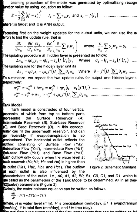
Prediction of future water availability required Etp series data, to get the data was conducted by ANN model. Input learning process of ANN in the form of climates parameter covering temperature, humidity, wind speed, and sun shine duration, while output is ETp result of measurement with pan evaporation. Scheme of ANN model for ETp prediction presented Figure 3.

Input layer

Hidden Iayer

Temperature

RH

Wind velocity

[image:9.600.91.454.269.383.2]

Sun Shine duration

Figure 3. Scheme of ANN Model for ETp Prediction

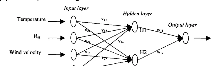
The prediction of future ETp (2004 to 2010) that is performed by an ANN model having as input past meteorological data observations (1990 to 2002) and as ouput future ETp values. Data used for input model ANN is totalizing ETp 10 year. Data study input is totalizing daily ETp 10 first year, and output is totalizing daily ETplO next year. For example, totalize 10 first year are totalizing ETp year 1989 to 1999 used as input, while output is totalizing ETp year 1990 to 2000. Follow the example of the calculation ETp year 2004 shall be as follows: data input model ANN is totalizing daily ETp year 1993 to 2003 ( contribution of each year to totalizing can be calculated percentage), while output is totalizing daily ETp year 1994 to 2004 or as totalizing daily ETp 10 year which is predicted. Daily ETp year 2004 is multiplication between totalizing ETp result of prediction with daily percentage year 1994. Predicted ETp used learning of ANN model again, is so that got value of weight different. The learning process continues to be conducted got ETp year 2010. Scheme learning of ANN model for prediction of total daily ETp 10 year presented at Figure 4.

Hidden Iayer Input layer

Total ETp ( I 0 years)

"-0-

Figure 4. Scheme of ANN Model for 10 years daily ETp prediction.

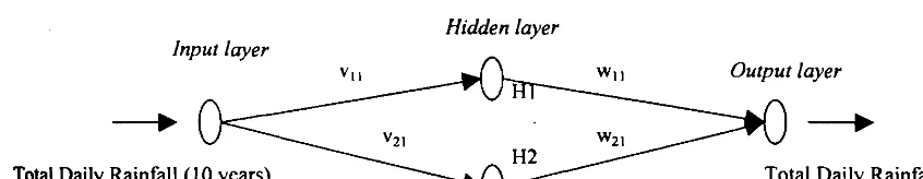
Rainfall Prediction

'The prediction of future rainfall (2004 to 2010) that is performed by an ANN

model having as input past rainfall data observations (1990 to 2002) and as ouput

future rainfall values. Scheme learning of ANN model for prediction of total rainfall 10

[image:10.598.37.460.85.167.2]

Hidden layer

Figure 5. Scheme of ANN Model for 10 years daily rainfall prediction.

ANALYSIS OF RESULTS

Data recorded by C'TD-DIVER logger is fluctuation of pressure due to water e of underwater ssure and free on the air as control. Data of Logger the analyzed is recorded ssure difference underwater logger and free logger on the air (Pw-Pa). The graph depicting relation between pressure and river water level presented at Figure 6 Stream discharge time to time was calculated by equation 1 dan Figure 6. The depth

of runoff caculated by equation 2 and 3. The depth of runoff (Figure 7) used for the

analysis of determination of tank model parameters in Ciriung sub-catchment.

l o -

y=1.1679r-18.837

101 151 201 251 301

15 17 I D 21 23 25 27

Pw-Pa (cm WC) Day

Figure 6. Presure vs water level Figur 7. The Runoff depth

According to three errors indicator that is RMSE, MAE, and LOGARITHM there four models having mistake indicator values which is small. Penman model, and Turc model. Penman model with Jensen-Haise

AE

=

0,5515, LOGARITHM

=

0,0601), Penman with

MAE = 0,4031, LOGARITHM = 0,0597), and Penman

E = 0,3631, MAE = 0, 2937, LOGARITHM = 0,0682).

cator values, ad for the model have value of R~ the big

enoughness. Penman model with Jensen-Haise model assess R*

=

0.8599, Penman

with Hargreaves R~ = 0,9425, and Penman with I Turc model R~ = 0,9615. Four

model have value ( RMSE, MAE, LOG ) small and big R ~ , this matter indicate that the

models have same correctness to prediction ETP.Thereby to prediction ETp in Ciriung sub-catchment can be used by simple models which only requiring two dimates parameter that are air temperature and sun radiation. Relation between Penman models with Hargreaves model presented at] Figure 8. For the input of tank model the ETp corrected with crop factor (kc= 0.86). Value of ETp corrective

presented at Figure 9.

0 ' 2 4 6 8 q O

I Hargreaves Yodel (rnrnlda).) 1 51 101 151 201 251 30 1

[image:11.598.46.505.66.214.2] [image:11.598.130.415.340.454.2]

I Day

Figure 8. Penman model vs Figure 9. ETc of C~r~ung sub-catchment July 2002 to June 2003 Hargreaves model

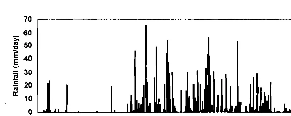
Rainfall data

The parameters of Tank models determined with daily rain data input. Daily

1

rainfall data got by automatic recorder from July 202 to June 2003. The rainfall data of Ciriung sub-catchment used for the input of tank model presented at Figure 10.

I

Figure 10. Rainfall data of Ciriung sub-catchment July 2002 to June 2003

Tank Model

The Optimization Technique was tested to determine the parameters of the Standard Tank Model in Ciriung sub-catcment; daily data of rainfall, evapotranspiration, and water discharge were well from July 2002 through June 2003. Table 1 shows the optimum parameter after going through optimization process for Ciriung sub-catchment. At the catchment, the Standard Tank Model resulted in very good water balance where the occurred discrepancy approaching

zero. As such, the coefficient of correlation ( R ) was over 0.82, whilst the other error

[image:11.598.149.409.649.736.2]

indicator was almost less than one e x c e ~ t for RMSE which was over 1 re~ectivelv

Table 1. Parameters of tank model Ciriung sub-catchment No Parameter Nilai No Parameter Nilai

1 Ao 0,047 7 c 1 0,001

2 A1 0.002 8 Dl 0,001

3 A2 0,025 9 Hal 15,OO 4 BO 0.006 10 H a2 60,OO

5 B 1 0,012 11 Hbl 0.001

[image:12.598.93.361.70.189.2] [image:12.598.76.397.272.471.2]

R RMSE MAE LOG SM.X S t d X A 2 RE RR

Figure 11. Performance indicators of tank model in Ciriung sub-

catchment

Figure 12 shows the hydrographic for Ciriung River. Ciriung River in theearly

r

shows somewhat high discharges. But in the middle of the year starting from the

June up to the early December of 2002 (dry season), it shows a decreasing rges. Here, the Standard Tank Model seems to be successful in approaching

ak discharges as compared to its nearness to the low discharges.

Figure 12. Hydrograph for Ciriung sub-catchment in 200212003

Rainfall and ETp Prediction

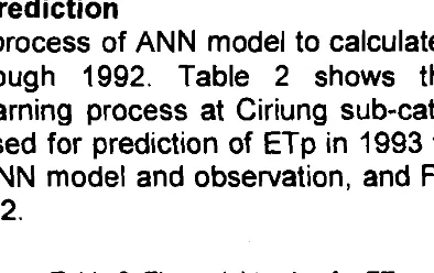
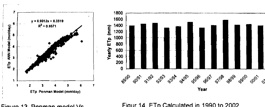
The learning process of ANN model to calculate ETp used climates parameter

data in 1990 through 1992. Table 2 shows the weight value after going backpropagation learning process at Ciriung sub-catchment in 1990 through 1992. The weight value used for prediction of ETp in 1993 through 2002. Figure 13 shows

the

verification of ANN model and observation, and Figure 14 shows ETp calculated

Table 2. The weight value for ETp prediction in 1992 to 2002

r

Weight Value Weight Value

V11 -0,22875 ~ 2 3 -1,01520

1

RMSE = 0,000893

1

[image:12.598.133.330.608.732.2]

D 2 1 b

&?'

&'

%a?' %-$' %+% '9d% 9896 4ffe %9q9 94~Q Q4\~Z

1 2 1 4 5 6 7

ETp Penman Model (rnrnlday) Year

F~gure 13 Penman model Vs F~gur 14 ETp Calculated In 1990 to 2002

ANN model

The future ETp (2004 through 2010) calculate based on the past ETp (1990

through 2002). Data of ETp used learning process of ANN model is 10 year totalizing

daily ETp. The training data used three sets data that are 1989 to 1999, 1990 to 2000, and 1991 to 2001. Table 3 shows the weight value after going backpropagation learning process with 10 year totalizing daily ETp, and Figure 15 shows the

verification ANN model and calculated. The learning process continues to be

conducted, then the result for prediction of ETp next year. Table 4 shows the weight value after going backpropagation learning process for prediction of ETp in 2004 through 2010, Figure 16 shows ETp in 2004 through 2010

Table 3 We~ght value for tralnlng data 10 year totaliz~ng

Pembobot Nlla~

VII -2,0672

1,9248 v21

-3,7432 w11

W12 1,3222 26 T0t.1 3 0 ETp 0 2 4 2 6 ca10uImled 40 46 (mm) 60

RMSE 1,17E-03

F~gure 15 ANN model vs calculated (Total~zlng ETp 10 years )

Table 4 The we~ght value for pred~ct~on ETp In 2004 through 2010

For pred~ction

We~ght 2004 2005 2006 2007 2008 2009 2010

VII 2,3620 1,5612 -1,4167 -1,3323 1,8699 -1,3424 1,6166 V21 -2,2239 -0,9656 1,7957 1,5850 -1,4866 1,7286 -1,4546 WII 1,511 32 0,9856 -2,4351 -2,0268 1,2099 -2,1688 1,1452 WZI -4,2453 -1,6672 1,1786 1,0930 -2,5228 1,1286 -2,2452

RMSE 0,0002 0 0054 0,0030 0,0039 0,0027 0,0037 0,0032

[image:13.598.43.482.64.242.2] [image:13.598.82.428.563.698.2]

[image:14.599.48.382.60.220.2]

03/04 04/05 05/06 06/07 07/08 08/09 09/10 Year

Figure 16. ETp in 2004 through 2010 Ciriung sub catchment

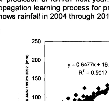
The future rainfall (2004 through 2010) calculates based on the past rainfall

(1990 through 2002). Data of rainfall used learning process of ANN model is 10 year

totalizing daily rainfall. The training data used three sets data that are 1989 to 1999, 1990 to 2000, and 1991 to 2001. Table 5 shows the weight value after going backpropagation learning process with 10 year totalizing daily rainfall, and Figure 15

shows the verification ANN model and calculated. The learning process continues to

[image:14.599.196.381.405.577.2]

be conducted, then the result for prediction of rainfall next year. Table 6 shows the weight value after going backpropagation learning process for prediction of rainfall in 2004 through 2010, Figure 17 shows rainfall in 2004 through 2010.

Tabel 5. Nilai pembobot hujan 10 tahun

Weight Value 250

1-7

CONCLUSION

1. The seven models were applied to determine ETp based on daily climatic data collected in one year using automatic weather station located at the Ciriung sub cacthment.The error indicators to evaluate the effectiveness of the ETp models are Root Mean Square Error (RMSE), Mean Average Error

(MAE), and Logaritmic RMSE (LOG), and the determination coefficient ( R ~ ) . The result shows that Hargreaves model is the most effective along with Turc and Jensen-Haise models.

2. The optimization technique to Tank Model gained fast and accurate results of total flow and flow components

3. Results revealed that the ANN networks were able to well learn the events

they were trained to recognize. Moreover, they were capable of effetively generalize their training by predicting potential evapotranspiration for sets of unseen cases. The ANN can forecast rainfall and evapotranspiration when trained on adequetely representative data set

4. Result of tank model analysis and ANN model was able to clarify water

availability in sub-catchment of Ciriung in dry season. Thus, irigated field area can be acounted.

ACKNOWLEDGEMENT

REFERENCES

Capece, J.C, Catteneo D, Lim Y.S, Rodriguez E.E, Upham L, Campbel K.L. 2002. Comparison of Evapotranspiration Estimation Methods. http://www.Southern- DataStream.com. [ I 2 Mei 2003]:35 p

Chow, V.T, D.R. Maidment, and L.W.Mays. 1988. Applied Hydrology. McGraw-Hill Book Company. London.

Doorenbos, J., and W.O. Pruitt. 1977. Guideline for Predicting Crop Water Require- ment. FAO.Rome. 144 p

Fukuda, T. et a/. 2001. Water Mangement and water Quality of Paddy Area Cidanau

Watershed at West Java. Prociding of 1'' Seminar Toward Harmonization between Development and Environmental Conservation in Biological Production February 21 -23, 2001 .Tokyo. Japan

u, L.M. 1994. Neural Network in Computer Intelligence. McGraw-Hill,lnc. New York.

eryansyah, A.2001. Aplikasi Model Tangki Pada Aliran Limpasan dan Kualitas Air untuk Manajemen Tata Guna Lahan di DAS Cidanau.Thesis. Pascasarjana

,

G.Y., T. Yano and K. Momii. 1998. An Improved Methodology to Measure

Evaporation from Bare Soil Based on Comparison of Surface Temperature with a Dry Soil Surface. J. Hydrol. 21 0, 93-1 05

Raupach, M.R. and J.J. Finnigan, 1997. The Influence of Topography on

Meteorological Variables and Surface-atmosphere Interactions. J. Hyeol. 190,

182-21 3

Setiawan, B.I.,T.Fukuda and Y.Nakano. 2003. Developing Procedures for Optimi- zation of Tank Models Parameters. Agricultureal Engineering International: the ClGR Journal of Scientific Research and Development. Manuscript LW 01 OOG.June, 2003.

Sugawara, M. 1961. On the Analysis of Runoff Structure about Several Japanese River. Japanese Journal of Geophysic. Vol 4 No. 2. The Science Council of Japan

Sutoyo, Purwanto,M.Y.J., Yoshida,K. and Goto,A. 2000. Prediction of River Runoff based on Rainfall Data using Tank Model in Cidanau Watershed. Proceding of International Seminar on Environmental Management for Sustainable Rural

Life.Bogor. February 19 'h.2000.

Toth, E., Brath H. 2002. Flood Forcasting Using Artificial Neural Networks in Black- Box and Conseptual Rainfaal-Runoff Modelling. http://www.iemss.org/-

iemss2002/proceedinqs/pdf/volume%20due/370 toth. pdf [3 Agustus 20031.6~ Wu, I.P. 1997. A Simple Evapotranspiration Model for Haeai: The Hargreaves Model.

CTAHR Sheet Engeineer's Notebook no.16 May 1997