Interpreting sensory data by combining p

(1)

Interpreting sensory data by combining principal component analysis

and analysis of variance

Giorgio Luciano

a

, Tormod N

s

a,b,* a_{NOFIMA FOOD, Matforsk, Oslovegen 1, 1430 Ås, Norway}

b_{Department of Mathematics, University of Oslo, Blindern, Oslo, Norway}

a r t i c l e

i n f o

Article history: Received 13 June 2008

Received in revised form 15 August 2008 Accepted 19 August 2008

Available online 11 September 2008

Keywords: PCA ANOVA Sensory profiling ASCA

a b s t r a c t

This paper compares two different methods for combining PCA and ANOVA for sensory profiling data. One of the methods is based on first using PCA on raw data and then relating dominating principal com-ponents to the design variables. The other method is based on first estimating ANOVA effects and then using PCA to analyse the different effect matrices. The properties of the methods are discussed and they are compared on a data set based on sensory analysis of a candy product. Some new plots are also pro-posed for improved interpretation of results.

1. Introduction

Sensory panel data can always be looked upon as three-way data tables with assessors, objects/samples and attributes as the three ‘‘ways”. In order to analyse differences and similarities be-tween samples and assessors as well as the correlation structure among attributes, the three-way structure of the data needs to be taken into account. This can be done in various ways using dif-ferent underlying ideas and philosophies.

A technique that can be useful in some cases is regular multi-variate analysis of variance (MANOVA, Kent & Bibby, 1978) for testing the effect of samples and/or assessors for all attributes simultaneously. Usually one is, however, interested in more insight than this method can give and therefore other techniques are to be preferred. A much used method within the area of sensory analysis is the generalised procrustes analysis (GPA), treating each assessor slice as a matrix, followed by a principal component analysis of the average or consensus matrix (Dijksterhuis, 1996). GPA is based on the idea of making individual assessor data matrices as similar as possible to each other by scaling and rotation. Another possible ap-proach is regular principal components analysis (PCA) of all indi-vidual sensory profiles followed by a two-way ANOVA of the most important components with assessor and products effects as independent variables. (Ellekj

_{r, Ilseng, & N}

_{s, 2002}_{). The rows}

in the data table used for this analysis correspond to all sam-ples * assessor combinations and the columns correspond to

sen-sory attributes. This method can be modified using the 50–50 MANOVA (Langsrud, 2002) method which handles significance testing in a more elegant way. Using partial least squares regres-sion (PLS-2) of all sensory profiles versus the two independent de-sign variables assessors and products and their interaction is a closely related approach (Martens & Martens, 2001). PCA based on the alternative unfolding with objects and assessor * attributes as columns and rows has been tested in for instance Dahl and N

s (2006). In the same paper a generalised canonical correlation analysis CCA (Carroll, 1968) analysis of individual sensory data was tested and compared to PCA. Classical three-way factor analyses such as Tucker-2 and PARAFAC have also found useful applications within the framework of sensory analysis (Bro, Qannari, Kiers, N

s, & Frøst, 2008; Brockhoff, Hirst, & N

_{s, 1996}_{). Recently an}

alterna-tive method for three-way analysis of variance (ANOVA) has been proposed in the chemometric literature (ASCA,Jansen et al., 2005), but the method is not yet tested for sensory data. ASCA is a method which first uses regular two-way ANOVA for each attribute sepa-rately, estimates the effects (under regular ANOVA restrictions) and then uses PCA on the main effects matrices and interaction matrix separately for interpretation of results. The method has re-cently been combined with PARAFAC in the so-called PARAFASCA (Jansen et al., 2008). Other important approaches and overviews of alternative methods can be found inQannari, Wakeling, Cour-coux, and MacFie (2000, 2001)and inHanafi and Kiers (2006).

The present paper is a comparison study of two of the ANOVA based methods described above. In particular we will be interested in comparing the newly developed ASCA method with traditional PCA of the unfolded three-way data table followed by ANOVA (here

* Corresponding author. Tel.: +47 64 97 0333; fax: +47 64 97 0165. E-mail address:tormod.naes@matforsk.no(T. Ns).

Contents lists available atScienceDirect

Food Quality and Preference

(2)

called PC-ANOVA). As can be noted, the two methods are closely related in the sense that they are both based on the same two basic methodologies, two-way ANOVA and PCA, but with the difference that the two methodologies are used in opposite order. These ap-proaches have the advantage over other methods that they focus both on the multivariate aspects of the sensory profiles and the ex-plicit relation of the sensory data to the design of the study. The methods will be compared conceptually and also with respect to results obtained in an empirical illustration.

2. Theory

In the present paper we will consider a three-way data table withI*Mrows corresponding toMreplicates ofIsamples,K col-umns corresponding to the attributes and withJslices correspond-ing to assessors. We refer to Fig. 1 for an illustration of the structure of the data set.

Three way data of this type can always, for each attributek, be modelled by the two-way ANOVA model

Xk

ijm¼

l

kþ

a

ki þbkjþ

ab

kijþekijm ð1Þ

Here the

l

is the general mean, the

a’s are main effects for products,

theb’s main effects for assessors, the

ab’s the interactions and

eis the random error term corresponding to replicate variation. For ANOVA purposes, the error terms are assumed to be uncorrelated and normally distributed with the same variance. The usual way of applying this model is to assume that the assessor and interac-tion effects are random, leading to a mixed model (see N

_{s &} Langsrud, 1998).

Sometimes experimental designs are used for the samples and in such studies (Baardseth et al., 1992), the product effect can be split in several components corresponding to the experimental fac-tors in the design (Box, Hunder, & Hunter, 1978). How to handle this extension within the framework of the methodologies pre-sented here will be discussed below. How to handle structures in the replicates will also be discussed in the same sections.

In the following we will use the symbolXto denote the un-folded three-way data table with I*M*J rows and K columns. Using this symbol it is possible to rewrite the model in Eq.(1) for all the attributes simultaneously as follows

X¼1

l

t

þD1B1þD2B2þD12B12þE ð2Þ

where

l

is the general mean vector for all K attributes simulta-neously, 1 is a vector of 1’s, theD1, D2andD12are the dummy

de-sign matrices for the products, assessors and interactions between assessors and products respectively and theB’s are the correspond-ing parameter matrices. TheB1corresponds to the

a’s in Eq.

(1), the

B2to theb’s andB3to the

ab’s. The design matrix

D1will have one

column for each assessor and consists of 0’s and 1’s with a 1 in col-umnjand rowiif this line corresponds to an observation for assessor

j. The same structure holds for the other two matrices. The matrixEis the matrix of residuals. Correlations between the different elements (columns) of this matrix are possible (Mardia, Kent, & Bibby, 1978), but it is always assumed within multivariate ANOVA that the error terms for different observations and replicates are independent.

The model (2) can be used directly, either for each attribute (column) separately or for all simultaneously for testing hypothe-ses about product and ashypothe-sessor effects. An example of an important hypothesis related to this model is H0:B1=0, which is the

hypoth-esis of no product effects. For the univariate ANOVA, this hypothe-sis can be separated in K individual hypotheses, one for each attribute. Similar hypotheses can be set up for assessor and inter-action effects. If wanted, one can also construct a combined hypothesis of for instanceB1andB12as is done in the ASCA paper

(Jansen et al., 2005) and inN

s & Langsrud, 1998.

The main problems with regular ANOVA approaches is that they only focus on hypothesis tests and provide little further insight about the relations between the attributes. Therefore ANOVA will usually be accompanied with some type of PCA for further inter-pretation of the relations between the variables. In this paper we will discuss two alternative approaches proposed in the literature for providing this type of additional insight by combining ANOVA with PCA.

For the purpose of the methods to be discussed below, it is of interest to estimate the effects matricesBin Eq. (2)above. This is usually done by least squares (LS) fitting of the responses to the design matrices, but in order to obtain unique results, one needs to add a restriction on the parameter estimates (see e.g. Lea, N

s, & Rødbotten, 1997). This can be done in various ways, but the most common way is to use the restriction that all main ef-fects of assessors and main efef-fects of products sum to 0 and that the same is true for the interactions summed either over assessors or products. In this paper main attention will be given to balanced designs, but how to extend the approach to more general data sets will also be discussed. For the balanced case, the main effects and interactions have a particularly simple expression based on simple averages and subtraction, i.e.

^

a

k

i ¼Xki Xk ð3Þ

^

bkj ¼Xkj Xk ð4Þ

a

^ bkij¼X

k

ijXki Xkj þXk ð5Þ

where_Xk

i is the average for productiand attributek,Xkj is the aver-age for assessorjand attributek. and_Xk _{is the total average for} attributek. Note that the interactions can be considered as obtained by double centring of the original data matrix.

When PCA is used in this paper we will always use it on centred data, i.e. data for which the average has been subtracted for each column.

2.1. PCA-ANOVA

The simplest way of combining ANOVA with PCA is to use PCA directly on the unfolded data matrixXin Eq.(2)where the number of columns corresponds to the number of attributes and the num-ber of rows corresponds to all assessor, product and replicate com-binations. This implies that the PCA gives components that are combinations of all the effects in the model (2). A possibility is to average over replicates before computation of principal compo-nents, but generally this is not natural since the replicates are needed for testing purposes in the subsequent ANOVA. Examples of the use of this and similar methodologies can be found in Ellekj

r et al. (2002)and inLangsrud (2002).

Attribute

Sample

Assessor

(3)

The PCA model, with let use sayAcomponents, for this data set (mean centred) can be written as

X¼TPT

þE ð6Þ

where T now represents theA first scores for the M*I*J prod-uct * assessor combinations andPrepresents the loadings for the

Kattributes for the same components. The Erepresents the rest, i.e. the components with small variance, sometimes thought of as noise. If we sort theXmatrix according to assessors (in the vertical direction), the firstI*_M_{rows of}_T_{will contain the scores for all the} products for the first assessor, the nextI*Mlines will contain the scores for all observations for assessor 2 etc. A similar sorting can be done for the samples.

As soon as the scores are computed, they can be interpreted by the use of scatter plots and also related to the design matrix using regular two-way ANOVA. The ANOVA model for the scores can be written as in Eq.(2)withXreplaced byT. All calculations of effects and hypothesis tests are done as for regular ANOVA. Since the

T- scores are uncorrelated, running separate ANOVAs for each re-sponse can now be justified. For exact statements of joint signifi-cances etc. they can, however, should also be considered in a joint approach.

The scores in Eq.(6)can always be written as (using Eq.(2))

T¼XP¼ ðD1B1þD2B2þD3B3þEÞP ð7Þ

The last part of the equation clearly shows that the scores are functions of all the effects in the data table including the errors

E. Note also that the noise part ofT, i.e.EP, can be written as a lin-ear function of the original noise matrixE. Since the error terms contribution of the scores are linear functions of the original errors, there are reasons to expect an error distribution closer to the nor-mal for the principal components than for the original attributes.

The product, assessor and interaction effects can as above be computed from averages of theT’s. For the purpose of improved interpretation of the multivariate variability in the data and its relation to the design variables we will in this paper propose to plot these effects in the same PCA scores plot as the original obser-vations (see alsoLangsrud, 2002). This is done by simply plotting the factor effects for the different components against each other in the PCA scores plot. For instance for the main effects for prod-ucts, the estimated

a

values (see Eq.(3)) obtained by ANOVA of score 1, are plotted against the corresponding estimated

a-values

for score 2. Note that this is identical to doing the corresponding averaging overX-values, projecting these averages ontoPand then plotting them in the same way as for the original scoresT. This im-plies that it is meaningful to interpret them vs. the same loadings as used for the interpretation of the original scores.

Another feature that will be proposed here for enhanced inter-pretation of the scores plots, is the superimposition of line seg-ments in both plotting directions (for PCA) corresponding to the level of noise in the same two directions. In the plots presented here we use the square root of the residual error variance for the ANOVA models for his purpose. For component number 1 this means that we first compute the square root of the residual error variance for the ANOVA model of the first component vs. the de-sign variables and then present this value as a line segment along the first component. The line segment is centred at 0. The same is then done for component number 2. Alternatively, one can use the least significant difference (LSD) values from multiple testing using the same ANOVA model. In both cases, the line segments provide the user with a visual tool for getting a quick and direct impression of the importance of the effects seen in the plot.

Note that all the usual tools of ANOVA, such as different types of sums of squares and corresponding tests (Type 1, Type II sums of squares (SS) etc.) can be used also for thet’s. In this paper,

how-ever, with balanced data, all the SS-types will give the same results. It should also be mentioned that as in regular ANOVA, multiple comparison tests may be used for assessing which individual prod-ucts and assessors that are different from each other along the dif-ferent PCA directions. Combined hypotheses related toD1andD12

as proposed in N

_{s and Langsrud (1998)} _{and for ASCA (}_Jansen et al., 2005can also be used here. The method can also easily be ex-tended to situations where the product effect is composed of dif-ferent experimental factors, for instance according to a factorial design. A simple example where the product effect is composed of two experimental factors can be modelled as

Xk

ijlm¼

l

kþ/ k iþd

k l þb

k j þ/d

k ilþ/b

k ijþdb

k

ljþekijlm ð8Þ

Whereuanddare now the two experimental factors in the product design andbis as before the assessor effect. A three-way interaction is also possible to incorporate in the model. The PCA ofXgoes as be-fore and the ANOVA of the scoresTis performed by simply incorpo-rating an extra factor in the model. All tests and computations of main effects and interactions etc. go as usual.

Another extension which is easily handled by the PC-ANOVA is the use of more complex error structure as discussed in e.g.Lea et al. (1997). An example of such a structure is the quite common replicate error structure

dkimþekijm ð9Þ

where the d’s correspond to the systematic replicate effect within each product and thee’s correspond to the regular random error noise. This model is quite typical in situations where the same physical sample, i.e. a replicate within product) (for instance a fish) is served to all panellists. In such cases, each individual fish,

m, is a replicate within product (for instance a special treatment) and will thus correspond to one of the d-terms in Eq. (9). The superscripts and subscripts have the same meanings as before;k

denotes attribute,idenotes product,jdenotes assessor andm de-notes replicate. Multiplying this effect byP, one obtains a new er-ror vector with the same structure

d_imPþeijmP ð10Þ

The two error terms in the sum now represent the vectors of the error contributions in Eq.(9)for all attributes considered simulta-neously. In other words, one can easily see that the more complex error structure in Eq.(9)is split in the same way for the scores as for the original variables.

Imbalance with respect to the number of replicates is also sim-ple to handle. The same effects can be used in the model (see Eq. (1)) and the same ANOVA can be used with the appropriate correc-tion for the degrees of freedom. The calculacorrec-tion of the effects is, however, slightly more complex, but this is easily handled by mod-ern ANOVA programmes. In situations with missing product and assessor combinations the situation is more complex, but not more complex than for regular ANOVA. The problem is then how to de-fine and compute interaction and main effects. Different sugges-tion is proposed. One simple possibility is to eliminate the interactions, but this is not advisable for sensory data at least unless a pre-treatment has been done to reduce the scaling effect (Romano, Brockhoff, Hersleth, Tomic, & N

s, in press).

(4)

the dummy design variables as the independent variables. This method is also graphically oriented, but less developed when con-cerns significance testing.

There is also a close relation of PC-ANOVA to an extension of the Tucker-2 model proposed by van der Kloot and Kroonenberg (1985). The classical Tucker-2 model is one with both common scores and common loadings and can be written as

Xj¼TWjPTþE ð11Þ

where nowXjindicates assessor or slice number in the data matrix

inFig. 1. The model (11) assumes that the different assessors share the same dimensions and their relation to the external data, but it allows for different weight to the two dimensions, represented by the individual matricesWj. The modification proposed invan der Kloot and Kroonenberg (1985) is to relate the common product scoresTto external data, for instance a product design matrix as was done for the PC-ANOVA. Representing Tas a linear function of the external design variablesDfor the products, the model in (11) can be written as

Xj¼DBWjPTþE ð12Þ

whereBis a matrix of regression coefficients and theDis the design matrix for the products. Note that the way the assessors and prod-ucts combine in this model is different from the PC-ANOVA. Here the joint effect is a combination of an additive effect for the prod-ucts and a multiplicative effect for the assessors.

An obvious advantage of the PC-ANOVA is its simplicity and that it provides both significance tests based on ANOVA and visual tools for direct interpretation of the tests (main effects, interaction plots and multiple comparisons). The main disadvantage is that if the factors span different multivariate spaces, the number of com-ponents to interpret may be high.

2.2. ASCA

Compared to the PC-ANOVA, the ASCA method is based on reversing the order of the two operations ANOVA and PCA. The first step is to use the regular two-way ANOVA model for each attribute (model (1) above) and estimate the effects using the regular ANOVA restrictions (sum equal to 0 over the levels). Considering these values for all attributes at the same time gives us a matrix of effects for the samples (dimensionI*K), a matrix of effects for the assessors (J*K) and a three-way matrix (I*J*K) for the inter-actions. The two former are regular two-dimensional matrices and can then be analysed directly by the use of PCA. The latter is ana-lysed by the use of PCA (also so-called Tucker-1. seeTucker (1966)) on an unfolded matrix as described above. Three different ways of unfolding are possible, but here we will focus on the same unfold-ing as for the PC-ANOVA, i.e. the unfolded matrix has dimensions

I*M*JandK. Note that the matrices used in ASCA correspond to the estimated versions of the matricesB1,B2andB3in the model

(2) above. As an example, theB1matrix can be written as

^

B1¼

X1 1

X1 _XK

1

XK

: : :

: :

X1

I X1 XKI XK

0

B B B B B B @

1

C C C C C C A

ð13Þ

As an alternative to using Tucker-1 for the interactions one can use the PARAFAC as was suggested inJansen et al. (2008). This cor-responds to using the PARAFAC on the double centred matrix, i.e. after subtraction of main effects. The method is called PARAFASCA. Note that this approach is a direct extension to several dimensions of the approach proposed inMandel (1971).

The difference between ASCA and the PC-ANOVA approach is that here the averaging is taken before PCA, while above it was ta-ken after PCA. This is generally an advantage for ASCA since one obtains PCA plots which are focused on the different effects and not influenced by everything at the same time. It may thus possibly give clearer conclusions for each of the separate effects. As will be seen from the example below, however, the multivariate spaces spanned by the different effects are rather similar for this data set.

-25 -20 -15 -10 -5 0 5 10 15 20 25

-20 -15 -10 -5 0 5 10 15 20

PC 1 % exp var 74.69

1 2 3 4 5

-0.8 -0.6 -0.4 -0.2 0 0.2 0.4 0.6 0.8

-0.6 -0.4 -0.2 0 0.2 0.4 0.6

Transp

Acid Sweet

Raspb.

Sugar Bites

Hard Elastic

Sticky

PC 1 74.69 % exp var

a

b

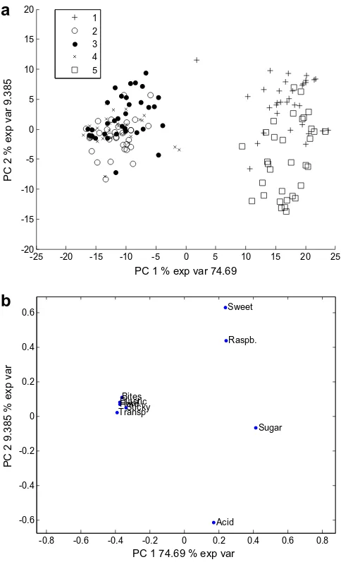
Fig. 2.PC-ANOVA. Scores and Loadings plot for component 1 and 2 of the unfolded sensory data.

Table 1

Percentage explained variance by the PCA model of the unfolded data organised as object * assessors * replicates vs. attributes

Number of components

Percentage variance explained

Cumulative percentage variance explained

1 74.69 74.69

2 9.38 84.08

3 6.47 90.55

4 2.90 93.44

5 1.98 95.42

6 1.89 97.30

7 1.28 98.58

8 1.08 99.67

9 0.33 100.00

(5)

Since no information about random variation is available in the plot, it is not obvious how to make a direct assessment of signifi-cance of the differences between products or assessors along the different axes as could be done for the PC-ANOVA using multiple comparisons. A possible extension of ASCA would be to add some type of confidence ellipses based on for instance the bootstrap (see e.gPages & Husson, 2005). For the same reason it is natural to use MANOVA and individual ANOVA’s before the ASCA to pro-vide additional insight about significant effects that can be used to interpret the ASCA plots.

Regarding imbalance, the same as stated for the PC-ANOVA can be stated also here. Also with respect to more complex error struc-ture, the ASCA method can be used. The only modification that has to be done is that a restricted maximum likelihood (REML) esti-mate is needed for improved estimation of effects. REML is a meth-od that takes the more complex error structure into account when estimating the effects. The standard LS estimates can also be used since they are unbiased, but the REML estimates are more precise. Also incorporation of factorial designs in the product structure is possible. As long as the effects can be estimated, the method can be used. One simply ends up with more than three matrices to sub-mit to PCA. For instance in the model (8) above, one will end up with 6 different PCA analyses. As the number of factors increases, the number of plots also increases. The ASCA method can also be used to analyse the joint effect of for instance the main effects of products and the interactions as was demonstrated in Jansen et al. (2005).

3. Data set

The data set chosen for this paper is from sensory analysis of a candy product. 5 different candies (I= 5). There areK= 9 sensory attributes andJ= 11 assessors in the panel and M= 3 replicates. The attributes were transparency, acidity, sweet taste, raspberry flavour, sugar coated texture tested with a spoon, biting strength in the mouth, hardness, elasticity in the mouth, stick to teeth in the mouth.

All variables were tested using a two-way ANOVA (model (1)) and all attributes were found to be significant for the separation of the samples and therefore kept during the study.

4. Results and discussion

All calculations were performed using MinitabÓ_{, 15}

Unscram-blerÓ 9.2 and custom made Matlab/Octave routines which are freely available for download from the first author’s website http://www.chemometrics.it.

4.1. PC-ANOVA

As can be seen fromTable 1, the explained variances are quite high for this data set (84% explained after 2 components). The first factor is totally dominating with a percentage of explained vari-ance equal to 75%. Scores and loadings plot of all the observations are presented inFig. 2. The scores are marked according to the 5 products. As can be seen fromFig. 2, there is some disagreement among the assessors, but the overall agreement among the assessors

Table 2

Mixed model ANOVA performed on components 1,2,3,4, (effect of assessors and interactions considered random and effect of sample considered fixed)

Source Sum Sq. d.f. Mean Square

Square root of mean square

F Prob >F

PC1

Assessor 224.9 10 22.49 1.27 0.2789

Sample 31470.6 4 7867.65 444.68 0

Assessor * sample 707.7 40 17.69 1.75 0.0116 Error 1109.3 110 10.08 3.17

Total 33512.5 164

PC2

Assessor 278.3 10 27.83 1.06 0.4166

Sample 1573.83 4 393.457 14.94 0

Total 4210.61 164

PC3

Assessor 1006.62 10 100.662 8.32 0

Sample 307.12 4 76.78 6.35 0.0005

Total 2902.38 164

PC4

Assessor 108.27 10 10.8275 1.21 0.313

Sample 29.62 4 7.4041 0.83 0.5149

Total 1299.21 164

All three replicates included in the analysis.

-25 -20 -15 -10 -5 0 5 10 15 20 25

-20 -15 -10 -5 0 5 10 15 20

1 2 3 4 5

-25 -20 -15 -10 -5 0 5 10 15 20 25

-20 -15 -10 -5 0 5 10 15 20

1 2 3 4 5

a

b

(6)

and replicates seems to be quite good for each product as compared to the difference between the products. The first component distin-guishes between two groups of objects, objects 2, 3 and 4 on one side and objects 1 and 5 on the other. The latter group has more sugar flavour, higher sweetness, raspberry and acidity taste, while the former group has more stickiness, hardness, transparency etc. The second axis primarily distinguishes between samples 1 and 5 and 3 and 5. Objects 2 and 1 are the less acidic and the sweetest and most raspberry flavoured among them. All the results were in accordance with what could be expected from the design of the samples.

As can be seen from the ANOVA tables inTable 2, the sample ef-fect is the dominating efef-fect for both the first two components, while for the third component, the assessor effect is the strongest. For the fourth component, none of the effects are significant. ANOVA was also conducted for the rest of the components with some significant effects here and there, but these results are not considered further here due to their very low explained variance (less than 5% in total). The interaction effect is significant for both the first components.

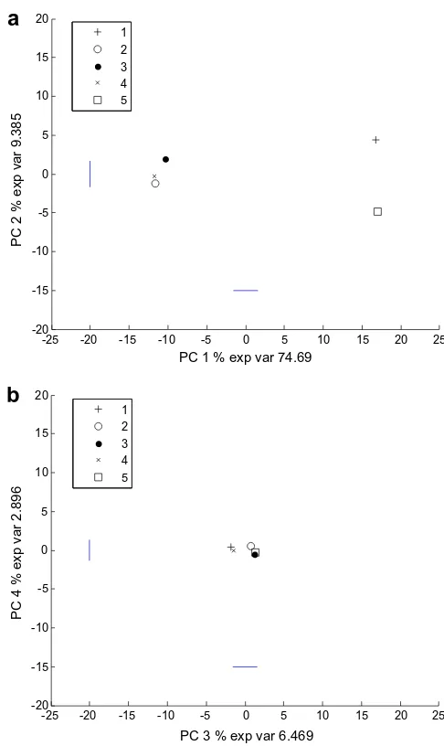
All these results correspond well to what is seen in the plots (Figs. 2–5). The advantage of the plots, however, is that one

automatically sees which samples those are similar and also their relation to the attributes. The product and assessor effects (see Eqs. (3)–(5)) are plotted along the same axes and with the same units as for the original scores. These results are presented inFigs. 3–5. The Fig. 3represents the products and shows a very clear tendency. As compared to the square root of the corresponding MSE, i.e the stan-dard deviation of the noise (presented as a straight line around 0 in both directions), one can also get a visual interpretation of the dif-ferences as compared to the noise level. Multiple testing (Tukey’s method) of the second axis (vertical) inFig. 3a, shows that sample 1 is significantly different from all except sample 3 and that sample 2 is only slightly different from 5 and not significantly different from the rest. The only sample which is significantly different from all is sample 5. For this data set, the average score plot of the prod-ucts does not provide new insight as compared to the overall plot, but in a more complex situation with several more objects and smaller differences between them this type of plot may simplify interpretation considerably. InFig. 4is presented the differences among the assessors and as can be seen, the differences are much smaller than for the product effects. Along the third axis there is some more variability among the assessors, however, which is also reflected in theF-test for assessors (Table 2).

-25 -20 -15 -10 -5 0 5 10 15 20 25

-20 -15 -10 -5 0 5 10 15 20

1 2 3 4 5 6 7 8 9 10 11

-25 -20 -15 -10 -5 0 5 10 15 20 25

-20 -15 -10 -5 0 5 10 15 20

1 2 3 4 5 6 7 8 9 10 11

a

b

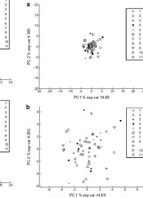
Fig. 4.PC-ANOVA. Plots of scores averaged over samples after performing PCA on the raw data. The horizontal and vertical bars close to the centre represent the squares root of the MSE.

-25 -20 -15 -10 -5 0 5 10 15 20 25

-20 -15 -10 -5 0 5 10 15 20

PC1 % exp var 74.69

1 2 3 4 5 6 7 8 9 10 11

-6 -4 -2 0 2 4 6 8

-6 -4 -2 0 2 4 6

1 2 3 4 5 6 7 8

10 11

a

b

Fig. 5.PC-ANOVA. PCA performed on data after double centring. Point is marked according to assessors. Figure b is a magnification of the figure a.

(7)

The interaction plot in Fig. 5is presented both for the same units as above and for units showing the results more clearly. The main advantage of the interaction plot is probably that it can shed some light onto which assessors that are the most similar to the average and which are the most different. It is for instance clear here that all points belonging to assessor 8 lie close to the centre of the plot while assessor number 10 has some of the points far away from the centre. This means that assessor 8 is much closer to the panel average for all the samples than assessor number 10. The latter is then more responsible for the interaction effect than assessor number 8. More specifically, one can also identify for which assessor and product combinations the interactions are larg-est. Comparing this with the loadings plot one can also obtain information about which attributes that are involved in the interactions.

A study of the normality of the residuals of the original data and the PCA scores was done according to the ideas mentioned in Sec-tion2.2. Generally, the residuals from the scores have a distribu-tion closer to normality than the residuals from the original variables. Two examples are presented inFig. 6a and b. inFig. 6a is given a typical example related to one of the original variables

(stickiness) while in Fig. 6b is presented the normality plot for the residuals from the ANOVA of the first principal component. As can be seen, the plot for the latter follows a much straighter line than for the former except from a few outlying points on each side.

4.2. ASCA

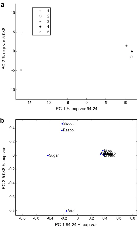
The product plots, assessor plots and the interaction plots are presented inFigs. 7–9. For the products inFig. 7, more or less the same interpretation as for the PC-ANOVA can be made. The plot is almost identical except for a 180 degrees switch of the first com-ponent which has no effect on the interpretation. Since no random variability is directly related to the plot, it is, however, hard to tell what is significant, in particular along axis 2. For the assessors plot inFig. 8, one can see that there are strong similarities between the loadings plot here and the loadings plot inFig. 7, indicating much of the same structure in the multivariate differences between the assessors as between the products. There are, however, some small differences related to for instance the attribute sugar coating. This may indicate a possible advantage of the ASCA. It is, however, hard to tell from the scores plot whether these differences are signifi-cant or not. For the interaction plot inFig. 9, the same as stated above is the case for the loadings. The interaction scores plot can be used for the same purpose as above. Again we see that assessor

-3 -2 -1 0 1 2 3

-8 -6 -4 -2 0 2 4 6 8 10

Standard Normal Quantiles

Quantiles of Input Sample

QQ Plot of Sample Data versus Standard Normal

-3 -2 -1 0 1 2 3

-15 -10 -5 0 5 10

Standard Normal Quantiles

Quantiles of Input Sample

QQ Plot of Sample Data versus Standard Normal

a

b

Fig. 6.Normal probability plot for (a) stickiness and the (b) first principal component.

-15 -10 -5 0 5 10

-10 -5 0 5 10

1 2 3 4 5

-0.8 -0.6 -0.4 -0.2 0 0.2 0.4 0.6 0.8

-0.8 -0.6 -0.4 -0.2 0 0.2 0.4

Transp

Acid Sweet

Raspb.

Sugar

Bites Hard_Elastic Sticky

a

b

(8)

number 8 is much closer to the average than is assessor number 10. The main conclusion is that for this data set, the two methods gave practically the same results and interpretations.

The fact that all the three matrices give similar loadings is strongly related to the fact that so few components are needed for the PCA on the raw data (PC-ANOVA), In a situation with differ-ent multivariate structure for the differdiffer-ent model effects, the num-ber of components for PC-ANOVA would basically be a sum of the dimensions for each of the effects and this is clearly not the case here. An interesting research question is whether this finding is generally true for sensory data.

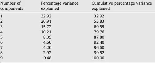
For the two main effects plots, 99% and 70% of the variation is explained by the first two axes while for the interaction plot, the corresponding value is 54% (SeeTables 3–5).

5. Conclusions

In this paper we have compared two approaches for analysis of sensory data which combine PCA and ANOVA. One of them is based on PCA of for the original data with subsequent ANOVA of the scores to test the effects of the design factors on the scores (PC-ANOVA). The other one is based on using PCA on the matrices of estimated main effects and interactions (ASCA). The difference

-3 -2 -1 0 1 2 3 4 5

-3 -2 -1 0 1 2 3

1 2 3 4 5 6 7 8 9 10 11

-0.6 -0.4 -0.2 0 0.2 0.4 0.6 0.8 1

-0.6 -0.4 -0.2 0 0.2 0.4 0.6

Transp

Acid

Sweet Raspb. Sugar

Bites Hard Elastic

Sticky

a

b

Fig. 8.ASCA. PCA scores and loadings plots for the assessor effects matrix.

-6 -4 -2 0 2 4 6

-5 -4 -3 -2 -1 0 1 2 3 4

1 2 3 4 5 6 7 8 9 10 11

-0.6 -0.4 -0.2 0 0.2 0.4

-0.4 -0.3 -0.2 -0.1 0 0.1 0.2 0.3 0.4 0.5 0.6

Transp

Acid Sweet

Raspb.

Sugar Bites

Hard

Elastic Sticky

a

b

Fig. 9.ASCA. PCA scores and loadings plot for the interactions data matrix.

Table 4

ASCA. Percentage variance explained by PCA performed on matrix of assessor effects

1 55.21 55.21

2 16.42 71.63

3 14.34 85.96

4 6.30 92.26

5 5.00 97.26

6 1.44 98.71

7 0.87 99.57

8 0.25 99.83

9 0.17 100.00

Table 3

ASCA. Percentage variance explained by PCA performed on matrix of products effects

1 94.24 94.24

2 5.09 99.33

3 0.58 99.90

4 0.10 100.00

(9)

between the methods lies in the fact that they use ANOVA and PCA in opposite order. Both methods have a multivariate focus since they consider all attributes simultaneously and they provide infor-mation about assessor effects and products effects as well as their interactions on the multivariate structure. In this sense both meth-ods are highly useful for analysing sensory data. Both methmeth-ods are easily computed using regular statistical software packages and none of them need any iteration or other complex numerical pro-cedures. Complex replicate structure and several factors in the experiment can also easily be handled without modification of the methods. Relations to other methods in the literature were highlighted in the method section.

The main advantage of PC-ANOVA is that it is easier to use for direct assessment of significant differences, also multiple compar-ison, directly related to the interpretation plots, i.e. PCA plots, ob-tained. Another advantage is that the PCA plots can easily be equipped with additional information that can be used to give a di-rect assessment of the size of the effects as compared to the noise level in the data, as measures by either the standard deviation of the random noise or the LSD values from multiple comparisons. The main disadvantage of PCA-ANOVA is that in cases where the different effects have a different multivariate profile, one may end up with many PCA components to analyse and interpret which can be both a time-consuming and complex task. This is particu-larly true in situations with several factors in the design. This is ex-actly the point where ASCA has its main advantage. Since it provides a separate PCA plot for each factor separately, each of the PCA models will generally have a lower dimension than for PC-ANOVA. Testing significance for the effects in the plots, is, how-ever, less obvious for the ASCA, although some recent attempts have been made to create such tests (Vis, Westerhuis, Smilde, and van der Greef (2007)).

As was demonstrated in the example, the two methods gave the same overall interpretation for this particular data set. It was de-tected that the assessor differences and product differences spanned the same low-dimensional multivariate correlation struc-ture leading to very similar loadings plots for the different effects for the ASCA method. This phenomenon leads to a small number of important components also for the PC-ANOVA. If this is not the cases, the latter method will need several components and the ASCA will need a different interpretation for each of the effect matrices. An interesting problem to be investigated in the future is how often this situation occurs in practice in sensory analysis.

In the example, only product and assessor effects were consid-ered, but both methods discussed can be extended to situations with several design factors and complex replicate structure.

Acknowledgments

We would like to thank Norwegian Research Council (NFR) for financial support for this study. We would also like to thank Asgeir Nilsen and Grete Hyldig for making the data available to us.

References

Baardseth, P., Naes, T., Mielnik, J., Skrede, G., Hølland, S., & Eide, O. (1992). Dairy ingredients effects on sausage sensory properties studied by principal component analysis.Journal of Food Science, 57(4), 822–828.

Box, G. E. P., Hunder, W., & Hunter, S. (1978).Statistics for experimenter. NY: Wiley. Bro, R., Qannari, E. M., Kiers, H. A., N_{s, T., & Frøst, M. B. (2008). Multi-way models}

for sensory profiling data.Journal of Chemometrics, 22, 36–45.

Brockhoff, P. M., Hirst, D., & N_{s, T. (1996). Analysing individual profiles by} three-way factors analysis. In T. N_{s & E. Risvik (Eds.),}_{Multivariate analysis of data in} sensory science. Elsevier Science Publishers.

Carroll, J. D. (1968). Generalisation of canonical analysis to three or more sets of variables. Proceedings of the 76th convention of the American Psychological Association(vol. 3) (pp. 227–228).

Dahl, T., & N_{s, T. (2006). A bridge between Tucker-1 and Carroll’s generalised} canonical analysis. Computational statistics and data analysis, 50(11), 3086–3098.

Dijksterhuis, G. (1996). Procrustes analysis in sensory research. In T. Ns & E. Risvik (Eds.),Multivariate analysis of data in sensory science(pp. 185–217). Elsevier Science.

Ellekjr, M. R., Ilseng, M. R., & Ns, T. (2002). A case study of the use of experimental design and multivariate analysis in product improvement.Food Quality and Preference, 7(1), 29–36.

Hanafi, M., & Kiers, H. (2006). Analysis of K sets of data, with differential emphasis on agreement between and within sets. Computational statistics and data analysis, 51, 1491–1508.

Jansen, J., Hoefsloot, J., van der Greef, M., Timmerman, E., Westerhuis, J., & Smilde, A. K. (2005). ASCA: Analysis of multivariate data obtained from an experimental design.Journal of Chemometrics, 19(9), 469–481.

Jansen, J., Bro, R., Huub, C., Hoefsloot, J., van den Berg, F. W. J., Westerhuis, J., & Smilde, A. K. (2008). PARAFASCA: ASCA combined with PARAFAC for the analysis of metabolic fingerprinting data.Journal of Chemometrics, 22, 114–121. Langsrud, O. (2002). 50–50 multivariate analysis of variance for collinear responses. Journal of the Royal Statistical Society: Series D, 51, 305–317 (The Statistician). Lea, P., N_{s, T., & Rødbotten, M. (1997).}Analayis of variance of sensory data. J. Wiley

and sons.

Mandel, J. (1971). A new analysis of variance model for non-additive data. Technometrics, 13(1), 1–18.

Mardia, K., Kent, J., & Bibby, J. (1978).Multivariate analysis. UK: Academic press. Martens, H., & Martens, M. (2001).Multivariate analysis of quality: An introduction.

UK: Wiley Chicester.

Ns, T., & Langsrud, Ø. (1998). Fixed or random assessors in sensory profiling?Food Quality and preference, 9(3), 145–152.

Pages, J., & Husson, F. (2005). Multiple factors analysis with confidence ellipses: a methodology to study the relationships between sensory and instr8umental data.Journal of Chemometrics, 19, 138–144.

Qannari, E. M., Wakeling, I., Courcoux, P., & MacFie, H. J. H. (2000). Defining the underlying sensory dimensions.Food Quality and preference, 11, 151–154. Romano, R., Brockhoff, P. B., Hersleth, M., Tomic, O., & N_{s, T. (in press) Correcting}

for different use of the scale and the need for further analysis of individual differences in sensory analysis, Food Quality and Preference, doi:10.1016/ j.foodqual.2007.06.008.

Tucker, L. R. (1966). Some mathematical notes on three-mode factor analysis. Psykometrica, 31, 279–311.

Van der Kloot, W. A., & Kroonenberg, P. M. (1985). External analysis with three-mode principal component analysis.Psykometrika, 50(4), 479–494.

Vis, D. J., Westerhuis, J. A., Smilde, A. K., & van der Greef, J. (2007). Statistical validation of megavariate effects in ASCA.BioMed Central (BMC) BioInformatics, 8, 322.

Table 5

ASCA. Percentage variance explained by PCA performed on the interaction effects

1 32.92 32.92

2 20.91 53.83

3 15.72 69.55

4 10.21 79.76

5 8.05 87.80

6 4.60 92.40

7 4.20 96.60

8 2.92 99.52