Coherent covariance analysis of periodic

(1)

Signal Processing 87 (2007) 13–32

Coherent covariance analysis of periodically correlated

random processes

I. Javors’kyj

a,b

, I. Isayev

a,c,

, Z. Zakrzewski

b

, S.P. Brooks

c

a_{Karpenko Physico-mechanical Institute of the National Academy of Sciences of Ukraine, Naukova St. 5, 79601, L’viv, Ukraine} b_{Institute of Telecommunications, University of Technology and Agriculture, Al. Prof. S.Kaliskiego, 7, 85-796, Bydgoszcz, Poland}

c_{Statistical Laboratory, Cambridge University, Wilberforce Road, CB3 0WB, Cambridge, UK}

Received 6 February 2005; received in revised form 13 April 2006; accepted 13 April 2006 Available online 5 June 2006

Abstract

A coherent method of estimating of periodically correlated random processes (PCRP) is introduced. Properties of estimates of the mean, covariance function and their Fourier coefﬁcients that are obtained using process values averaging over the period are investigated. Asymptotic formulae for estimates of bias and variances are obtained and the relationships of these characteristics to realization length are discussed. The probabilistic structure of one of the simplest PCRP-based signals is analysed.

Keywords:Periodically correlated random processes; Mean; Covariance function; Coherent estimation; Bias; Consistency

1. Introduction

Recurrence and stochasticity are characteristic features of many physical processes exhibiting time changeability[1–3]. Recurrence of process properties could be caused by the inﬂuence of external forces (e.g., forced oscillations) acting on the system or from internal forces (e.g., autonomous oscillation) that exist within the system itself. Rhythmic processes occur in many ﬁelds including radio physics[4], telecommunications[3], geophysics [5], oceanography [1,2], meteorology [6–9], vibro-diagnostics [10,11], biology [12,13] and seismology[14,15], for example. The methodological basis for investigating rhythmic process structure based on experimental data is the mathematical model. Early investigations into rhythmic processes were based on deterministic models using periodic and almost-periodic functions. Attempts to describe the stochastic changeability of oscillations were enhanced by the evolution of probabilistic methods based mainly on models in the form of stationary random processes. Rhythmic changeability of physical processes is evidenced by the oscillatory character of the associated correlograms and also in the peak values present in spectral density estimates. However, these characteristics describe only time-averaged oscillatory properties. They have no www.elsevier.com/locate/sigpro

_{Corresponding author. Cambridge University, Statistical Laboratory, Wilberforce Road, CB3 0WB, Cambridge, UK. Tel.: +44}

(0)1223 766925; fax: +44 (0)1223 337956.

(2)

information about the time structure of any oscillations, which might be introduced, at least in idealized form, by the incorporation of additional deterministic structure, for example. The development of probabilistic models such as PCRP and their generalizations (bi-, poly- and almost-PCRP) is the natural evolution of these approaches[1–4,16–18]. These models generalize the idea of recurrence to situations where stochasticity plays a dominant role in the system process and they enable us to make more detailed and objective descriptions of stochastic recurrence including, as special cases, the earlier models described above. PCRP models also enable us to analyse the properties of physical processes without needing to specify special characteristics of the process a priori,but provide a generic method for identifying characteristics present in the underlying process. Suppose that we have a time series xð Þt, t2R then this series is said to be periodically stationary with periodTif

Pr½xðt1þhÞ 2A1;xðt2þhÞ 2A2;. . .;xðtnþhÞ 2An ¼Pr½xðt1Þ 2A1;xðt2Þ 2A2; :::;xðtnÞ 2An

forh¼T40, and no smaller value ofh.

PCRP (or cyclo-stationary) models are deﬁned uniquely by the speciﬁcation of a mean function mðtÞ ¼

ExðtÞ;t2 ½0;TÞ and a covariance function bðt;uÞ ¼ExðtÞxðtþuÞ; for t2 ½0;TÞ and u2R, where

x t

ð Þ ¼xð Þ t m tð Þ. Analysis of PCRP process models therefore involves estimation of these two functions. PCRP means,m(t) and covariance functionsb(t,u) are periodic functions of time and ifR₀Tm tð Þdto1and

RT

0 b tð;uÞdt

o1,u2R, then they can be represented by the Fourier series:

m tð Þ ¼ X

k2Z

mkeiko0t

¼m0þ

X

k2N

mc_kcosko0tþmsksinko0t

ð1Þ

and

b tð;uÞ ¼X

k2Z

Bkð Þu eiko0t¼B0ð Þ þu

X

k2N

Bc_kð Þu cosko0tþBskð Þu sinko0t

; (2)

respectively. Hereo0¼2p=T;mk¼1₂ mckimsk

;Bkð Þ ¼u 1₂ Bckð Þ u iBskð Þu

and bothjmkj !0 and Bkð Þu

!

0 ask! 1. The parametersBk(u) are referred to as thecovariance components [1,2,17],coefficient function

[19]or the cyclic autocorrelation function[3,16]. The Fourier components are also commonly of interest and their estimation often forms part of the analytic process.

An important part of understanding the properties PCRP’s is the PCRP decomposition into stationary connected random processes[1–3], or harmonic serial representations[3]

xð Þ ¼t X

k2Z

xkð Þteiko0t, (3)

where the xk(t) denote stationary connected random processes. The characteristics of the signal x(t) can therefore be derived from the corresponding characteristics of the constituentxk(t) processes.

Nomenclature

x(t),xk(t),Z(t) stochastic signals

T period

y realization length

E sign of mathematical expectation

m(t) mean function

m_k mean components

b(t,u) covariance function B_k(u) covariance components

(3)

Various methods have been proposed for the estimation of the mean and covariance functions. For example Isayev and Javors’kyj[6]investigates the use of component methods, whereas Javors’kyj et al. [20]develop approaches based upon least squares estimation. In this paper, we will focus on the so-called coherent method estimation, proposed by Gudzenko [4]. The coherent method (also known as synchronized averaging[16]) is based on averaging sample PCRP realization values at the same point across different periods to obtain empirical estimates of the mean and covariance functions. For example, since yis an integer multiple of the period,T, the coherent estimate of the mean has the form:

^

m tð Þ ¼ 1

N

X N1

n¼0

xðtþnTÞ fort2½0;TÞ. (4)

Several authors have used the coherent method for analysing PCRP processes. In this paper, we focus on the properties of the corresponding estimators. We begin in Section 2 by looking at the coherent estimators of the mean function and the corresponding Fourier series components and demonstrate their unbiasedness and consistency. In Section 3, we prove the asymptotic unbiasedness and consistency of the covariance function before doing the same for the corresponding Fourier components in Section 4. In Section 5, we conclude with an example in which we investigate the properties of the signal corresponding to a particular implementation of the PCRP process.

2. Properties of the PCRP mean function and corresponding component estimators

The coherent mean function estimator in (4) is clearly unbiased since

Em t^ð Þ ¼ 1

N

X N1

n¼0

m tð þnTÞ ¼m tð Þ.

To prove consistency, we need to show thatD½m t^ð Þ !0 asN! 1. We begin by noting that

D½m t^ð Þ ¼E½m t^ð Þ Em t^ð Þ2¼ 1

N

X N1

n¼Nþ1

1j jn

N

b tð;nTÞ. (5)

The proof is trivial.

D½m t^ð Þ ¼ 1

N b tð;0Þ þ2

X N1

n¼1

1 n

N

b tð;nTÞ

" #

(6)

and, if

lim

N!1 1 N

XN

n¼1

b tð;nTÞ ¼0, (7)

thenD½m t^ð Þ !0 asN! 1. Thus, the estimator in (4) is also consistent. Note that condition (7) is satisﬁed if the sumPN_n_¼₁b tð;nTÞincreases withNno faster thanNa_{, where}_ao_{1. Note also that condition (7) is evident if} limj j!1u bðt;uÞ ¼0.

Taking into account the foregoing we now formulate the following theorem:

Theorem 1. Statistic (4) is an unbiased and consistent estimate of the PCRP mean if condition (7) is satisﬁed, its variance being deﬁned by expression (6).

The variance (6) is a periodic function of time with corresponding Fourier series expansion:

D½m t^ð Þ ¼g₀þX

l2N

gc_lcoslo0tþgsl sinlo0t

. (8)

From (2), we therefore have that:

g₀¼ 1

N B0ð Þ þ0 2

X N1

n¼1

1 n

N

B0ðnTÞ

" #

(4)

and

Similarly, from (2) and under the condition in (7), we have that:

lim

The zero componentg0deﬁnes the average value of the variance of the coherent estimator (8) and depends only upon the zero covariance componentB0(u). Thelth harmonic components which deﬁne the amplitudes of the variance D½m t^ð Þ depend only on the covariance components of the same order. If correlations vanish within a time interval less than the period T (i.e., if B0ðnTÞ ¼Blc;sðnTÞ ¼0 for all n40), then expressions Let us now consider the estimation of the Fourier components corresponding to the mean function given in (1). Suppose, that the mean estimate m t^ð Þ, is known for all t2 ½0;TÞ. Then we can create the following

Combining (4) and (12), we obtain:

^

To demonstrate consistency of the component estimates, we note that

D½m^0 ¼

See Appendix A for details. Settingu¼stwe obtain:

(5)

and

Finally, substituting b(t,u) for its Fourier series decomposition in (18) and integrating with respect tot, we obtain large ywe have

D½m^0

Using similar manipulations, (19) and (20) become

Dm^c_l¼2

If the following conditions

lim

are satisﬁed, then the variances in Eqs. (21)–(23) vanish asy! 1. Thus the estimators in (12) are consistent as well as asymptotically unbiased.

Taking into consideration the foregoing we now formulate the following theorem:

Theorem 2. The statistics in (12) are unbiased and consistent estimates of the PCRP mean Fourier coefficients if the conditions in (24) are satisfied, their variances being defined by the expressions in (21)–(23).

It is clear from Eq. (21) that the zero covariance component is the main characteristic deﬁning the variance of the zeroth-order mean estimate. The variances of higher-order mean estimates are functions both of the zero component and the components of double their order i.e., Dm^s_l;c depends bothB0 and on Bs₂;_lc. The constituent sine and cosine components in (22) and (23) have opposite signs. Therefore, the variance of the complex amplitude estimateD½m^l ¼1₄ D m^cl

þD m^s_l

is independent of higher covariance components, i.e.,

D½m^l ¼

The dependence of this variance on the valuelclearly stems from the frequency of the cosine weight function.

3. Properties of the covariance function estimators

The coherent covariance function estimate is given by

^

Suppose that the realization length is such that y¼NTþum, where um denotes the maximum lag of the

(6)

^

The proof follows directly from a similar expression to that given in (5).

Foru¼0 this expression differs from the variance of mean estimate, given in (5), only by the sign. Clearly, changes in the covariance function directly affect the bias. Therefore we can obtain a Fourier series representation similar to that forD½m t^ð Þgiven in (8) i.e.,

coherent estimator in (25) is asymptotically unbiased.

Let us obtain the variance of estimate (25) under the assumption that the PCRP is Gaussian (so that third and higher-order moments can be expressed in terms of ﬁrst and second-order moments), and then rewrite (25) in the form

Then, since third and higher-order moments can be expressed in terms of ﬁrst and second-order moments under the Gaussian assumption, as a ﬁrst order approximation we get:

Dhb t^ð;uÞi¼ 1

The proof follows similarly to that given in Appendix A.

(7)

Then, using the fact that b tð;uÞ ¼b tð u;uÞit follows from (30) that

Theorem 3. The estimate of the covariance function (25) of a Gaussian PCRP is asymptotically unbiased and consistent if conditions (11) are satisﬁed and its bias and variance are deﬁned by the formulae in (27) and (32).

Let us represent the function bZðt;u1;uÞin terms of the Fourier series decomposition:

bZðt;u1;uÞ ¼

X

k2Z

~

Bkðu1;uÞeiko0t. (33)

Then, settingu1¼nT and substituting (33) into (32) we have that

Dhb t^ð;uÞi¼a0ð Þ þu

Using the earlier decomposition of the covariance functionb tð;uÞinto Fourier series, we can directly obtain expressions for the componentsB~lðu1;uÞ. Suppose that we haveMcovariance components, then we have from

(31) that

Thus from (34), we have that lim

u

j j!1D ^

b tð;uÞ

h i

¼0, the condition required to demonstrate the consistency of the estimator in (25).

From (35) it is clear that the average value of the variance in (34), corresponding to component a0ð Þu ,

depends on the zerothandall higher order covariance components. Thus, in the case of PCRP processes the precision of our estimates could not be obtained by looking at stationary processes alone.

4. Properties of the covariance component estimators

Let us now consider the coherent estimators for the covariance components. Suppose that the estimate

^

b tð;uÞis known for allt2 ½0;TÞand for allu2½0;um. Note that, in practice, we truncate our estimator for the

(8)

range, we can create the following estimates of the covariance components:

Taking into consideration expressions for bias of the covariance function estimates in Eqs. (28) and (29) and the Fourier decomposition of the covariance function in (2) we have, after integrating, that

B^0ð Þu

The biases of the covariance component estimates for any order depend only on the covariance components of the same order. If the conditions in equation (11) are satisﬁed then these biases clearly converge to zero as N! 1. Thus, the estimators in (38) and (39) are asymptotically unbiased.

In order to investigate consistency, we require expressions for the variances of the estimators in Eqs. (38) and (39). Combining Eqs. (38) and (39), using the deﬁnition ofb t^ð;uÞfrom (25) and the periodic property of the mean estimate i.e.,m t^ð þnTÞ ¼m t^ð Þ, we have that

For Gaussian signals we get a ﬁrst-order approximation:

DB^0ð Þu

Proof follows similarly to that given in Appendix A.

Substituting the Fourier decomposition of bZðt;u1;uÞ from (33) into Eqs. (40)–(42) and integrating with

respect tot, we obtain for largey (or, equivalently,N):

(9)

DhB^s_lð Þu i2

then the variances in equations (43)–(45) vanish as y! 1. Hence, we have asymptotic consistency for the estimators in Eqs. (38) and (39).

Theorem 4. Estimates (38)–(39) for Gaussian PCRP are asymptotically unbiased and consistent if the

conditions in (11) and (46) are satisﬁed and their biases_B^₀_{ð Þ}_u _¼₀_{ð Þ}_u _, _B^c

and variances are deﬁned by the formulae in (28)–(29) and (43)–(45).

Since valuesB~0ðu1;uÞandB~

c;s

l ðu1;uÞare evaluated through the PCRP covariance components products, the

conditions (46) hold if and only if the conditions in (24) hold true. The proof is trivial. The expressions in Eqs. (43)–(45) are similar to those for the variances of mean components in Eqs. (22) and (23). The difference is that we use the Fourier components of the functionbZðt;u1;uÞin the ﬁrst case and covariance components in the

second. It follows from (37) thatB~0ðu1;uÞdepends upon all covariance components. Hence, the accuracy of

the estimator for the zero covariance component B0(u) cannot be measured without considering the higher order covariance components. Once again, the variance of our estimators could not be obtained by looking at stationary processes alone. The variances of the sine and cosine covariance components depend also on the higher order components of the functionbZðt;u1;uÞ. However, for the variances of complex-valued estimates

^

Thus, the accuracy of the higher-order complex-valued covariance component estimates depend only on

~

B0ðu1;uÞ.

5. Characteristics of modulated signals—an example

As we saw in Section 1, Eq. (3), we can decompose our signal into a series of stationary connected sub-signals (harmonic serial representations) as follows:

xð Þ ¼t X

k2Z

xkð Þteiko0t;

where thexk(t) denote stationary random processes.

There are several common forms of constituent process. For example, if we setxkð Þ ¼t akþZkð Þt, where the Z_kð Þt are uncorrelated, then we get the additive model

xð Þ ¼t X

wheref(t) is a periodic function andZ(t) is a stationary random process. Such models are commonly used for simple processes with stochastic variation around a periodic mean.

If we set xkð Þ ¼t akZð Þt, then we get the multiplicative PCRP model, where xð Þ ¼t Zð Þt X

k2Z

akeiko0t¼f tð ÞZð Þt. (47)

(10)

A third model is obtained if wex1ð Þ ¼t 1=2½xcð Þ t ixsð Þtandx1ð Þ ¼t x1ð Þt, with the remaining stationary

processes all set equal to zero i.e.,xkð Þ t 0 forj jka1. In this case, we get the quadrature model that allows for

interactions between the stationary and quadrature components.

xð Þ ¼t xcð Þt coso0tþxsð Þt sino0t.

In this section, we take a speciﬁc example of a multiplicative model and investigate the properties of the signal for a particular form of periodic function and associated stationary random processes. We shall assume thatf tð Þ ¼coso0tin (47) and, using the properties of elementary circular functions, we obtain the following

mean and covariance functions

m tð Þ ¼mcoso0tandb tð;uÞ ¼B0ð Þ þu Bc2ð Þu cos 2o0tþBs2ð Þu sin 2o0t,

where

m¼EZð Þt; B0ð Þ ¼u Bc2ð Þ ¼u 1=2RZð Þu coso0u and Bs2ð Þu

¼ 1=2RZð Þu sino0u ð48Þ

andRZð Þu denotes the covariance function of stationary processZð Þt. In this case, and from (8) and (9), the bias of the mean equals zero and we get the following variance for the mean:

D½m t^ð Þ ¼g₀þgc₂cos 2o0tþgs2sin 2o0t,

where

g₀¼gc₂¼ 1

2N RZð Þ þ0 2

X N1

n¼1

1 n

N

RZðnTÞ

" #

,

and

gs₂¼0.

Now, suppose that we setRZð Þ ¼u Deaj ju, then we have that

g₀¼gc₂¼ D

2N½1þ2SðaT;NÞ, where

SðaT;NÞ ¼X

N1

n¼1

1n

N

eaTn¼ e

aT

1eaT 1

1eaNT N_ð1eaT_Þ

(49)

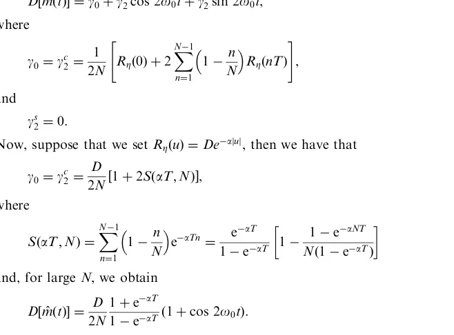
and, for largeN, we obtain

D½m t^ð Þ ¼ D

2N

1þeaT

1eaTð1þcos 2o0tÞ. (50)

Fig. 1plots the variance of the mean estimate as Nand tvary. This plot clearly demonstrates the rapid decrease in the variance D½m t^ð Þ as Nincreases. Note also that the variance in (50) vanishes at the points tk¼ð2kþ1ÞT=4,k2Z. This implies that the mean at the pointstkmust be known and is a consequence of the deﬁnition ofm(t) asm(t)¼mcoso0twhich clearly equals zero at the points tk.

As we saw in Section 2, the mean components can be deﬁned using a Fourier transform of the mean function. Here, we have only one componentl¼1 and so, from (21)–(23), it is simple to show that

D½m^0 ¼

D

NP1ðaT;NÞ; D½m^c ¼ D

NP2ðaT;NÞ; D½m^s ¼ D

N½2P0ðaT;NÞ þP2ðaT;NÞ, where

PlðaT;NÞ ¼

1 T

Z y

0

1u

y

eaj ju coslo0udu¼

1

a2_T2_þ_4l2_p2 aT

a2_T2_4l2_p2

Na2_T2_þ_4l2_p2 1e

aNT

" #

.

(11)

The productaTdenotes the rate of damping of the estimate variances withN.Fig. 2provides a plot of these variances asNchanges.

We now consider the properties of the estimate of the covariance function,b(t,u). Eqs. (27)–(29) suggest the following result for the bias:

jb t^ð;uÞk¼0ð Þ þu 2cð Þu cos 2o0tþs2ð Þu sin 2o0t,

where

0ð Þ ¼u c2ð Þ ¼ u

D

2NS0ðaT;N;uÞcoso0u;

s

2ð Þ ¼u

D

2NS0ðaT;N;uÞsino0u and

S0ðaT;N;uÞ ¼

X N1

n¼Nþ1

1j jn

N

eajuþnTj.

From (49) and for zero lag (i.e.,u¼0) we haveS0(aT,N,u)¼1+2S(aT,N). So, in analogy to the case for the components of the bias of the covariance function, expressions for the components e0(0) andec2(0) differ from the corresponding Fourier components of the mean estimate varianceg0andgc2only in sign.

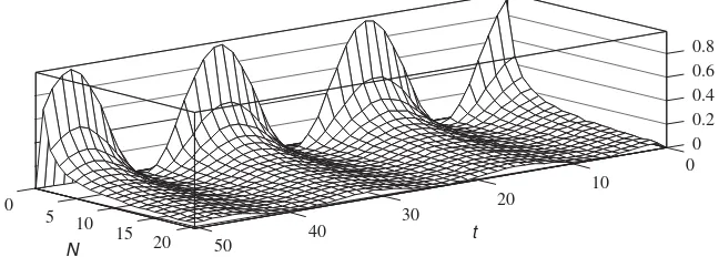
The functionS0(aT,N,u) oscillates but its amplitude decreases asuincreases. However, the damping rate is less than that for the covariance. This obviously affects the biasjb t^ð;uÞk(seeFig. 3) It is relatively easy to show that the relative valuehb t^ð;uÞi=b tð;uÞincreases with laguand, because the numerator is only defined over a finite range, it is possible to assess the reliability of the covariance function estimate only for lags within the finite interval [0,um].

0

5 ₁₀ 15

20

0 10

20 30

40 50

0

N

t

0.8

0.6 0.4

0.2

Fig. 1. Variance of mean estimate depending on period numbersNand timetforo0¼0.2,a¼0.1 andD¼1.

0 5 10 15 20

0 0.6

0.5

0.4

0.3

0.2

0.1

zero cos sin

(12)

We now examine the variance of the covariance function estimate. Using Eqs. (24), (48) and the properties of elementary circular functions, we obtain the following Fourier components of the functionbZ(t,u1,u) in (31):

~

B0ðu1;uÞ ¼1₈R~Zðu1;uÞð1þcos 2o0uþcos 2o0u1Þ,

~

Bc₂ðu1;uÞ ¼18R~Zðu1;uÞ½1þcos 2o0uþcos 2o0u1þcos 2o0ðu1þuÞ,

~

Bs₂ðu1;uÞ ¼1₈R~Zðu1;uÞ½sin 2o0uþsin 2o0u1þsin 2o0ðu1þuÞ,

~

Bc₄ðu1;uÞ ¼₈1R~Zðu1;uÞcos 2o0ðu1þuÞ; and; B~

s

4ðu1;uÞ

¼1

8R~Zðu1;uÞsin 2o0ðu1þuÞ,

whereR~Zðu1;uÞ ¼R2Zð Þ þu1 RZðuþu1ÞRZðuu1Þ. Similarly, from (34)–(36) we obtain the following expression

for the variance of the covariance function estimateb(t,u):

Djb t^ð;uÞk¼a0ð Þ þu

X

l¼2;4

ac_lð Þu coslo0tþaslð Þu sinlo0t

(52)

where

a0ð Þ ¼u

D2 8N

~

SðaT;N;uÞð2þcos 2o0uÞ,

ac₂ð Þ ¼u D

2

4N

~

SðaT;N;uÞð1þcos 2o0uÞ,

as

2ð Þ ¼ u

D2

4N

~

SðaT;N;uÞsin 2o0u,

ac₄ð Þ ¼u D

2

8N

~

SðaT;N;uÞcos 2o0u,

as₄ð Þ ¼ u D

2

8N

~

SðaT;N;uÞsin 2o0u,

and

~

SðaT;N;uÞ ¼1þe2aj ju þ2Sð2aT;NÞ þ2S1ðaT;N;uÞ,

S1ðaT;N;uÞ ¼

X N1

n¼1

1 n

N

eaðjuþnTjþjunTjÞ.

Componentsa0(u),ac2(u),a c

4(u) are even functions of laguanda s 2(u),a

c

4(u) are odd functions. Foru¼0, the componentsa0(u), a

c 2 (u), a

c

4(u) are bounded above, whilsta s

2(u) anda c

4(u) take the value zero. Thus

0

0 5 10₁₅

20

30

50

N

u

-0.2

-50 -30

-10

10

0.1

-0.1

(13)

Eq. (52) reduces to

Dhb t^ð;0Þi¼D

2

4N½1þ2Sð2aT;NÞð3þ4 cos 2o0tþcos 4o0tÞ

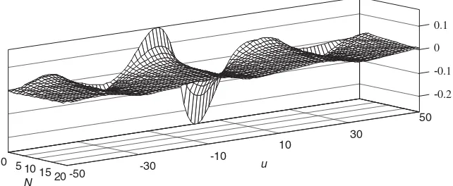
in this case. The variance of the covariance function estimate is plotted inFig. 4. Again, the valueDjb t^ð;0Þk

equals zero at the pointstk¼ð2kþ1ÞT=4 which can be explained by noting thatb tð;0Þ ¼D=2 1ð þcos 2o0tÞ.

The behaviour of all of the components take the form of damped oscillations for small lags. However, for

larger lags, the components converge to periodic functions. Thus, the variancesDjb t^ð;uÞkdo not vanish with increasing lag, but exhibit damped oscillatory behaviour. The amplitudes of these oscillations decrease withN

and the relative mean-square error

ffiffiffiffiffiffiffiffiffiffiffiffiffiffiffiffiffiffiffiffi

Dhb t^ð;uÞi

r

=b tð;uÞ grows rapidly with increasing lag. Thus, we use a simple process of correlogram cutting to obtain reliable estimates. Note also that the maximum truncation pointumincreases withN.

It is clear from Eqs. (37) and (52) that the undamped periodic tail of the variance for covariance function estimate is caused by non-stationary characteristics of the underlying signal i.e., the second covariance components Bc2(u) andBs2(u). From (37), the stationary contribution ina0(u) depends only on the stationary approximation of the covariance functionB0(u) and has the form

að Þ₀sð Þ ¼u D

2

8N½2 1ð þ2Sð2aT;NÞÞ þð1þcos 2o0uÞ e

2aj ju _þ_2S

1ðaT;N;uÞ

(see Appendix B).

For the non-stationary part, which depends on the higher-order component, we have

að Þ₀nð Þ ¼u D

2

8N e

2aj ju _þ_cos_o

0uþ2Sð2aT;NÞ

cos 2o0uþ2S1ðaT;N;uÞ.

Obviouslya0ð Þ ¼u að Þ₀sð Þ þu að Þ₀nð Þu and, foru¼0 we obtain

að Þ₀sð Þ ¼0 D

2

2N½1þ2Sð2aT;NÞ; a

n

ð Þ

0 ð Þ ¼0

D2

4N½1þ2Sð2aT;NÞ. For large uwe also have that

2

4N½1þ2Sð2aT;NÞ; a

n

ð Þ

0 ð Þ ¼u

D2

8N½1þ2Sð2aT;NÞcos 2o0u

Clearly,að Þ₀nð Þ0=að Þ₀sð Þ ¼0 0:5 and the same limit is reached by the equivalent ratio for large lag values. Thus, the non-stationarity component plays a signiﬁcant role in the analysis of estimation reliability. Elimination of the non-stationary components can lead to signiﬁcant error for all possible lags.

Finally, we investigate the properties of the covariance components estimates. Biases in these estimates have the same form as those for the corresponding Fourier components of the covariance function estimate. For the

0

20

40

60

0

10

20

30 0

N

u 0.3

0.2

0.1

(14)

variances, Eqs. (43)–(45) give us the following results:

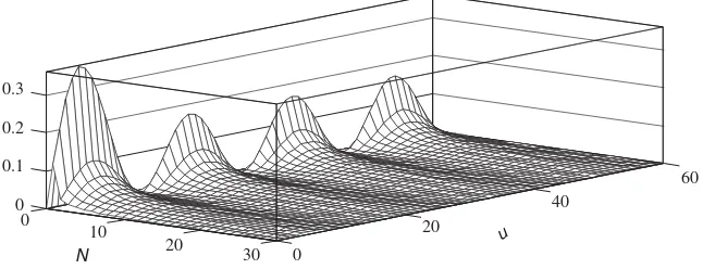
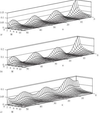
Fig. 5illustrates the cyclic variations in the functions given in Eqs. (53)–(55). These variations are caused by the periodic non-stationarity of the underlying signal.

For u¼0 the functions P~lðaT;N;uÞ and Plð2aT;NÞ are equal: i.e., P~lðaT;N;0Þ ¼Plð2aT;NÞ. There are

three distinct components to the expressions in Eqs. (53)–(55). The ﬁrst does not depend on lagu, the second component is damped with increasing lag and the third changes periodically with the lag. For the variance of the zeroth covariance component whenu¼0, we have

DB^0ð Þ0

¼D

2

2N½2P0ð2aT;NÞ þP2ð2aT;NÞ and for large lags we obtain

DB^0ð Þu ¼

D2

4N½P0ð2aT;NÞð1þcos 2o0uÞþP2ð2aT;NÞ (56)

sinceP~lðaT;N;uÞ !0 asu! 1.

Cyclic variations in the function given in (56) have large amplitude and substantially change the variance D B^0ð Þu

(seeFig. 5). These variations are caused by the presence of periodic stationarity in the signal. The variance in (41) can be split into two components (following similarly to the procedure shown in Appendix B): a stationary component;

Dð Þs B^0ð Þu

and a non-stationary component;

Dð Þn B^0ð Þu

(15)

Thus,Dð ÞnB^0ð Þ0=Dð ÞsB^0ð Þ0 X0:5 and the elimination of signal non-stationarity leads to signiﬁcant error

in calculating the variance of our estimate. For largeu, the stationary component is independent of lag, i.e.,

Dð ÞsB^0ð Þu¼

D2

4N½P0ð2aT;NÞ þP2ð2aT;NÞ, (61)

whereas the non-stationary component is a cyclical function of lag i.e.,

Dð Þn B^0ð Þu

¼ D

2

4NP0ð2aT;NÞcos 2o0u. (62)

The value of (61) is half as great as the starting valueDð Þs _B^

0ð Þ0

given in (59) and the amplitude of the cyclical oscillations of the non-stationary part in (62) is also half as great as that forDð Þn B^0ð Þ0

given in (60). Thus, the signal non-stationarity signiﬁcantly changes the variance of the estimate and also its as we change the lag, u.

It also follows from expressions (54)–(55), that the zeroth and second-order covariance components deﬁne the properties of the variances of the second covariance component estimates. For zero lag (i.e.,u¼0)

0 2 4 _{6 8} 10

0 10

20 30

40 50

0

N

u

u 0 ₂

4 6 _{8 10}

0 10

20 30

40 50

0

N

0 2 4 ₆ 8 10

0 10

20 30

40 50

0

N 0.15

0.1

0.05

0.2

0.1

0.05 (a)

(b)

(c)

Fig. 5. Variance of covariance components estimates: (a)DB^0ð Þu

(16)

we have

DhB^c₂ð Þ0 i¼D

2

2N½2P0ð2aT;NÞ þ4P2ð2aT;NÞþP4ð2aT;NÞ, (63)

DhB^s₂ð Þ0 i¼D

2

2N½2P2ð2aT;NÞ þP4ð2aT;NÞ (64)

and for large lags, we have

DhB^c₂ð Þu i¼D

2

4N½½P0ð2aT;NÞ þ2P2ð2aT;NÞð1þcos 2o0uÞ þP4ð2aT;NÞ, (65)

DhB^s₂ð Þu i¼D

2

4N½P0ð2aT;NÞð1cos 2o0uÞþ2P2ð2aT;NÞð1þcos 2o0tÞ þP4ð2aT;NÞ. (66) Variances (65) and (66) decrease by a factor of two relative to the initial values of the constant part given in (63) and the cyclic part in (64), respectively.

As the lag increases, the rate of decrease in the variancesDB^0ð Þu

,DjB^c₂ð ÞukandDhB^s₂ð Þu iis less than the corresponding decreasing rate for the covariance componentsB0ð Þu ,Bc2ð Þu andBs2ð Þu . This means that as the

lag increases, so do the corresponding relative mean-squares errors

ffiffiffiffiffiffiffiffiffiffiffiffiffiffiffiffiffiffiffi

D B^0ð Þu

q

=B0ð Þu

and

ffiffiffiffiffiffiffiffiffiffiffiffiffiffiffiffiffiffiffiffiffi

DhB^c₂;sð Þu i

r

=Bc_c;sð Þu. As before this limits the consistency of estimating the covariance component for lag values beyon0d the interval [0,um], though we note that the maximum lag value umgrows asNincreases.

6. Conclusions

One of the most significant tasks in the statistical analysis framework is the analysis of the reliability of estimators for quantitative indices of interest. Here, we investigate this task for the analysis of periodic stationary random signals. Obtaining quantitative indices makes it possible to justify the choice of process parameters. This is necessary for avoiding errors, understanding the model and for model verification. In this paper, the reliability of the so-called coherent process is investigated in terms of biases and variances of the non-stationary mean, covariance function and the corresponding Fourier components. The relationships we obtain show a dependence of both bias and variance on realization length and on the signal covariance components. On the basis of formulae for the covariance components for the partial PCRP cases, it is possible to investigate in detail the properties of these estimates and to obtain relationships between parameters of the stationary processes, which form the PCRP. The variances of the covariance characteristic estimates take the form of undamped oscillations as the lag increases. The amplitude of these oscillations is defined by characteristics of the signal non-stationarity and their average values are defined by the characteristics of the signal stationary approach. Such behaviour in the variance as the lag changes indicates that the reliable estimation of the covariance characteristics is possible only for lags within the range [0,um]. Within this interval, the variances of the estimates take the form of damped oscillations. Specific value for um can be calculated by means of the formulae we derive here.

Appendix A

Proof of consistency of the component estimates given in Eqs. (12).

D½m^0 ¼E½m^0Em^02¼E½m^0m02

¼E 1

y

Z y

0

x t

ð Þdt

(17)

¼ 1

After changing the order of integration, we have

D½m^0 ¼

Substituting heresfortuwe receive

D½m^0 ¼

Substituting here the Fourier decomposition of covariance function b(t,u), we have

D½m^0 ¼

If we deﬁne the function

f_lð0;yuÞ ¼1

. After substituting into the previous formula and cancelling, we obtain

(18)

Appendix B

From (37) we have

~

The ‘‘stationary part’’ of this equation depends only on zero covariance component and ‘‘non-stationary part’’ depends on covariance componentsB2ð Þu andB2ð Þ ¼u B2ð Þu:

Taking into account (48) we obtain

e

From (26) we have

(19)

Taking into account above expressions we obtain

2

8N e

2aj ju _{cos 2}_o

0uþ1

ð Þ

"

þ2þ2X

N1

n¼1

1n

N

eaðjnTþujþjntujÞðcos 2o0uþ1Þ þ2e2ajnTj

#

.

2

8N e

2ajnTj_þ_{cos 2}_o

0u

"

þ2X

N1

n¼1

1 n

N

e2aj ju cos 2o0uþeaðjnTþujþjntujÞ

#

.

And ﬁnally,

2

8N 2 1ð þ2Sð2aT;NÞÞ

þ e2aj ju þ2S1ðaT;N;uÞ

1þcos 2o0u

ð Þ,

2

8N e

2aj ju _þ_cos_o

0uþ2Sð2aT;NÞ

cos 2o0uþ2S1ðaT;N;uÞ,

where

SðaT;NÞ ¼X

N1

n¼1

1 n

N

eaTn,

S1ðaT;N;uÞ ¼

X N1

n¼1

1 n

N

eaðjuþnTjþjunTjÞ.

References

[1] Ya. Dragan, I. Javors’kyj, Rhythmics of Sea Waving and Underwater Acoustic Signals, Naukova dumka, Kijev, 1982 (in Russian). [2] Ya. Dragan, V. Rozhkov, I. Javors’kyj, Methods of Probabilistic Analysis of Oceanological Rhythmics, Gidrometeoizdat, Leningrad,

1987 (in Russian).

[3] W.A. Gardner, Cyclostationarity in Communications and Signal Processing, IEEE Press, New York, 1994.

[4] L. Gudzenko, On periodically nonstationary random processes, Radiotekh. Elektron, 6 (1959) 1062–1064 (in Russian). [5] E.R. Kanasewich, Time Sequence Analysis in Geophysics, The University of Alberta Press. Edmonton, Canada, 1981.

[6] I. Yu. Isayev, I. N. Javors’kyj, Component analysis for time series with rhythmical structure, Izvestija VUZov ‘‘Radioelektronika’’, No.1, 1995, pp. 34–45 (in Russian).

[7] Y. Kwang-Y, Statistical prediction of cyclostationary processes, J. Climate 13 (6) (1999) 1098–1115.

[8] D. Reynolds, T.H. Vonder Haar, A bispectral method for cloud parameter determination, Mon. Weather Rev. 105 (1977) 446–457. [9] D.J. Thomson, Time series analysis of Holocene climate data, Philos. Trans. R. Soc. Lond. A. 330 (1990) 601–616.

[10] A.C. Mccormick, A.K. Nandi, Cyclostationarity in rotating machine vibrations, Mech. Systems Signal Process. 12 (2) (1998) 114–131.

[11] P.D. Mcfadden, M.M. Toozhy, Application of synchronous averaging to vibration monitoring of rolling element bearings, Mech. Systems Signal Process. 14 (6) (2000) 891–906.

[12] M.J. Cassidy, W.D. Penny, Bayesian nonstationary autoregressive models for biomedical signal analysis, IEEE Trans. Biomed. Eng. 49 (10) (2002) 1142–1152.

[13] B. Upshaw, M. Rangoussi, T. Sinkjaer, Detection of human nerve signals using higher-order statistics, in: Proceedings of the 1996 8th IEEE Signal Processing Workshop on Statistical Signal and Array Processing, SSAP’96, Cortir, Greece, 1996, pp. 186–189. [14] K. Bullen, B. Bolt, An Introduction to the Theory of Seismology, Cambridge Press, Cambridge, UK, 1985.

(20)

[16] W.A. Gardner, The spectral correlation theory of cyclostationary time-series, Signal Processing 11 (1986) 13–36.

[17] E. Gladyshev, Periodically and almost periodically correlated random processes with continuous time, Probabilistic Theory and its Applications, vol. 3, 1963, pp. 184–189 (in Russian).

[18] O. Koronkievych, The linear dynamic systems under action of the random forces Nauk. Zap. Lvivskogo Univ. 44 (1957) 175–183 (in Ukrainian).

[19] H.L. Hard, Nonparametric time series analysis for periodically correlated processes, IEEE Trans. Inform Theory IT-35 (1989) 350–359.