DOI: 10.12928/TELKOMNIKA.v13i2.132 460
The Implementation of One Opportunistic Routing in
Wireless Networks
Li Han1,2*, Huan-yan Qian1 1
School of Computer Science & Technology, Nanjing University of Science & Technology, Nanjing, China, 210094
2
School of Computer Science & Technology, Anhui University, Hefei, China, 230039 *Corresponding author, e-mail: [email protected]
Abstract
In the paper, it proposes an optimization framework addressing fairness issues for opportunity routing in wireless mesh networks, where we use network coding to ease the routing problem. We propose a distributed heuristic algorithm in the case when scheduling is determined by MAC, and discuss the suitability of our algorithm through simulations. It is found that in most situations our algorithm has better performances than the single-path algorithm and the classical network coding which is based opportunity algorithm MORE.
Keywords: Opportunistic Routing, Network Coding, Utility, Suitability
1. Introduction
The application of wireless channels presents some unique opportunities that can be used to improve the performance. For example, the broadcast nature of the medium can be used to provide opportunistic transmissions just as suggested in the paper [1]. Also, in wireless networks, there are typically multiple paths connecting each source destination pair; using some of these paths in parallel can improve performance [2]-[4].We adopt an optimization framework to design a distributed maximization algorithm. We address questions of fairness by maximizing the aggregate utility of the end-to-end flows, where we associate a utility function U (·) with a flow. We use network coding [5] to simplify the problem of scheduling packet transmissions across multiple paths, which are similarly to papers [1],[3],[4],[6],[7].
However, the traffic along the multiple paths may interference along with adjacent paths in wireless network. Some way is needed to alleviate the side-effect of extensive exploration. In MORE [6] ,each node keeps a pre-statistics variable TX credit and a credit counter. When node i receives a packet from a node upstream, it increases the counter by its TX credit. When the 802.11 MAC allows the node used for transmitting, the node will check whether the counter is positive. If yes, the node will create a coded packet, and broadcasts it, then consume the counter. If the counter is negative, the node can not be used in the transmitting. NCMR [7] allowing a forwarder broadcast coded packet of a generation only when it has got all packets of the generation, but it does not work well in most situations. Both of the two algorithms do not give any guidance to handle multiple flows. The main contributions of the paper are as follows: (1) We propose a network wide optimization algorithm that maximizes rate-based global
net-work performance, and propose a primal-dual congestion control mechanism that can be implemented in a decentralized fashion for each flow.
(2) It uses the distance from the sending nodes to destinations as means to alleviate the side-effect of extensive exploration.
(3) Comparisons of our algorithm with MORE and a single-path routing algorithm used the same kind of jointly-optimal routing and flow-control approaches are made. Simulation results show that our algorithm outperforms the other two protocols in most situations.
2. Model
2.1. PHY and MAC Characteristics
We consider a network comprising of a set of nodes N,n N , with the set L of communication links between them that are fixed or time-varying according to some specified processes. There is a set of multicast sessions C sharing the network. Each session cC is associated with the set Sc N of source nodes, and set TcNSc of sink nodes.
The channel state vector S t( ) is assumed to be constant in each time slot t i.e., state transitions occur only on slot boundaries, where time t is an integer. We assume that in each time slot the value of S(t) is taken i.i.d. from a finite set; Let S be the set of S. it needs to decide which flow it will be transmitted through. It is defined through a flow scheduling profile matrix A. If node i transmits a packet from flow c , we setAic 1,
y t be the potential number of packets that are destined for
destination of flow c out i and into j; y tijc( )=0, if ( , )i j L.
c i
q is the number of packets that are destined to destination of flow c. The system is stable if every queue size is bounded. The rate vector f is valid under the following three conditions:
( ) 0
vector f is feasible, when coding generation size goes to infinity if and only if it belongs to F. Moreover, the set of feasible end-to-end rates F is convex.
3. Optimal Flow Schedule 3.1. Maximization of Utility
For each flowcC, we define a utility function U f( c) to be a strictly concave,
increasing function of end-to-end flow rate fc. The goal of utility maximization is to achieve trade-off between efficiency and fairness. We can write the network-wide optimization problem as:
Since set of F is convex and the objective is strictly concave, there exists a unique solution f of the maximization problem. Corresponding y also exist but are not necessarily unique. We can write the KKT conditions at the optimal point:
( )
Hence intuitively we can relate c i
to c i
q , the number of packets that are destined to destination of flow c. As a consequence of KKT, using some elementary algebra one can derive:
It can be found that the optimal scheduling rule (7) is an NP-hard centralized optimization problem. It should consider a more realistic, suboptimal scheduling process and we will show how our algorithm can be applied as a distributed heuristic.
A back-pressure between nodes iand j is defined as c c c ij i j
z q q , i can send packets
to jonly when c 0
ij
z .We call a set of feasible activation profiles S 802.11-compatible if for all
SS and for all ( ,i J1 1)S, there is no ( ,i J2 2)S such that pi i1, 2 0, or pi1,j 0 and pi2,j 0in
which j J1 J2. Furthermore, we will assume that the underlying scheduling process is not under our control. We can simplify the schedule to the Eq (8).
( , ) ( )
d d is used to alleviate the side-effect of extensive exploration. c i
Flow control: The optimal flow rate at the source f tc( ) can be calculated through using
a primal-dual approach as in the paper [8]:
least two times of the max link rate . 12
In this section we consider some practical issues that concern implementation of the Algorithm proposed in Section 3. Table 1 defines the terms used in the rest of the paper.
Table 1. Definitions used in the paper Term Definition
Native Packet Uncoded packet
Coded Packet Random linear combination of native or coded packets
Innovative Packet A packet is innovative to a node if it is linearly independent from its previously received packets
Downstream Node Let c
i
Only when forwarders accept at least thred native packets of a generation, it can relay re-encoded packets of the generation.
4.1. Network Coding
Previous results assume that generation size used for network coding tends to infinity. Practical reasons, such as complexity and performance of decoding, and header overhead for storing the coefficient vector, require us to limit the size of the header.
With random linear codes, data to be disseminated is divided into l packets b b1, 2...bl,
where each block bihas a fixed number of bytes h (referred to as the packet size). In order to code a new coded packets Xjin network coding, a network node should first independently and randomly choose a set of coding coefficients cj1,cj2...cjl in GF(2
8
), one for each received packet
(or each original packet on the data source). It then produces one coded block Xj of h bytes:
1
. Note that a linear combination of coded packets is also a linear combination of thecorresponding native packets.
Since each coded packet is a linear combination of the native packets, it can be uniquely identified by the set of coefficients that appeared in the linear combination. A peer decodes as soon as it has received l linearly independent coded blocks X X1, 2...Xl, let
1,... l
X X X . It first forms a l l matrix C, using the coefficients of each block Xi. Each row in C is correspond with the coefficients of one coded block. It then recovers the original block b ,
1, 2,..l
b b b b as 1 T
bC X . It should be noted that a network node does not have to wait for all l linearly independent coded blocks before decoding a generation. In fact, it can start to decode as soon as the first coded block is received, and then progressively decodes each of the new coded blocks, as they are received through the network. In this process, the decoding time overlaps with the time required to receive the original block, and thus hidden from the tally of overhead caused by encoding and decoding times. We use Gauss-Jordan elimination to implement such a progressive decoding process rather than the more traditional Gaussian elimination, which is also used as an effective method of innovative packet judgments.
4.2. Stopping Rule
(a) Once the source stops doing so. (b) The downstream nodes of it have got all packets of the generation. Eventually the generation will be timeout and be flushed from memory. (c) Additionally, forwarders that hear the ACK while it is being transmitted towards the sender immediately stop transmitting packets from that generation and purge it from their memory. (d)Finally, the arrival of a packet of a new generation will cause a forwarder to flush all buffered packets with generation IDs which is lower than the active generation.
In simulations, we find the timeout period of a generation on source node impact performance significantly. We use an algorithm similar to TCP protocol on each source to compute and manage timeout timer. However, we do not compute timeout timer for each packet but for each generation. We can calculate the timeout period RTO like this:
(1 ) , 0.125
s S Sample
RTT RTT RTT a (10)
(1 ) , 0.25
D D S Sample S
RTT RTT RTT RTT RTT (11)
4 S D
RTORTT RTT (12)
RTTSample is currently measured RTT, which is defined as the period from the source
sending the first packet of a generation till it accepting ACK of the generation from its destination. Where RTTS is the smoothed RTT of a generation; RTTD is the smoothed RTT
deviation. When a generation is timeout on a source, it will be flushed from the memory, and next generation should be sent.
In order to simplify the implementation and reducing control overhead, we assume only one generation is transmitted for a flow at once. Only generations having got at least thred+1 innovative packets and not meeting stopping rules, it can compete for scheduling chance with Eq (8). We call the resulting generation, if it exists, scheduling generation.
4.3 Control Flow
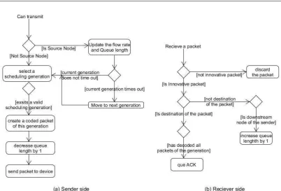
Figure 1 shows the architecture of our protocol. The control flow responds to packet reception and transmission opportunity signaled by the 802.11 driver. On the sending side, whenever the MAC signals has an opportunity to transmit, the node selects a backlogged flow as mentioned in section 3.2 and pushes its pre-coded packet to the network interface. If the node is a source, it should update its flow rate and queue length according to Eq.(9) first, and at the same time it should check whether current generation is timeout. On the receiving side, when a packet is arriving, the node checks if the generation ID in the packet is higher than the node’s current generation, the node sets current generation to the more recent generation ID and flushes packets of older generations from its generation buffer. If the generation ID on the packet is the same as its current generation, the node performs a linear independence check to determine whether the packet is innovative. Innovative packets are added to the generation buffer while non-innovative packets are discarded. If the packet was transmitted from upstream, the node will increases its queue length by one.
Figure 1. A flow chart of our protocol implementation
5. Simulation Results
We compared our algorithm with a shortest-path, single path routing algorithm, and with the MORE algorithm. In order to make the comparison fair, we assume that the single-path routing algorithm used the same kind of jointly-optimal routing and flow-control approach in our scheme. In contrast, MORE does not integrate flow control or flow scheduling with the routing algorithm. In the simulation of the MORE algorithms, we assume that each source had a large backlog of packets to transmit, and that each relay performed FIFO scheduling among packets from different flows. Algorithms assign the same size of buffer on each node. We name the single path protocol with SinglePro and our algorithm with MulPro in this section.
We developed a discrete-event simulator that implements the three routing, flow and rate control algorithms. In the simulations, the following settings are adopted: (a) The Distributed Coordination Function (DCF) of IEEE 802.11 for wireless LANs is used as the MAC layer protocols. (b) 40 nodes; Packet drop probability averages is 0.2 on each link; Link bandwidth is 4Mbps; Packet size is 1000 Bytes. (c) Parameters used in Eq(9) are defined as K=256, m= 0.05, M= 2.5. We use U f( c)log(fc), hence the rate allocation that maximizes Eq (4) is the proportionally fair rate allocation.
We looked at four performance metrics. (a) Total utility ( c) c
U f
: Allocation f' is better than f if ,( c) ( c)
c c
U f U f
Figure 2. Performance with various generation size l in a network with average 10 neighbors and 8 randomly selected flows
We first discuss the influence of generation size l. Figure 2 illustrates performance of MulPro and MORE with various generation size l, where thred equals l1. We can see all performance metrics are increased compared to MORE. We found that generation size has significant impact on the performance of MulPro, but that’s not the case for MORE. The negative influence of large size generation in MulPro is caused by the timeout mechanism used in source nodes, which needs quick decoding on destinations. This feature can help us reduce the overhead of network coding.
Figure 3. End-to-end rate allocation example: eight flows among randomly selected source-destination pairs on one network with average 15 neighbors for each node. Small bars denote
rates per flow.(l = 4, thred = 3 )
Figure 3 illustrates the optimal rate allocations obtained through our algorithm, Where
( Mulpro) 45 c
c
U f
, ( MORE) 36c c
U f
, Pr( Single o) 40 c
c
U f
. In this case, we can see that bothFigure 4. Cumulative performance improvement of our algorithm over SinglePro with various number of neighbors
The curve "Percent_utility" is the percentage of runs, in which
Pr Pr
( Mul o) ( Single o) 0 c c c c
c c
U f U f
. And the curve " Percent_rate" is percentage of flows thatsatisfy
Pr Pr 1
Mul o c Single o c
rate rate
We then make the previous experiments with 30 random traffic matrices for each network with various numbers of neighbors, and compare Mulpro to SinglePro with the two performance metrics which is illustrated in Figure 4. We can see Singlepro performs better with less number of neighbors, for MulPro can not take advantage of multiple paths in a sparse network. When the number of neighbors is between 6 to 18, it is observed that network utility of Mulpro wins in about 85% runs and throughput wins in about 70% flows.
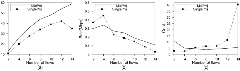
We now look at the influence of the number of flows, with the simulation results illustrated in figure 5. We can see from figure 5(a) that the rate allocation obtained by MulPro always maximizes the utility with the average delivery ratio over 90%. Figure 5(c) shows that the increasing number of flows has little negative effect on the cost of MulPro, but that’s not true for SinglePro.
Figure 5. Performance improvement of our algorithm over SinglePro with various number of flows in a 8-neighbor-network
6. Conclusions
coding, which help us to solve the routing problem. We get a distributed heuristic algorithm in the case when scheduling is determined by MAC, which is especially well-suited for multimedia applications with low-loss, low-latency constraints such as audio/video streaming. Through simulations, we have shown our approach significantly outperforms single-path routing and MORE in most situations. We also inspect the influence of different network conditions with experiments. The performance of applications that run on the top of our system is an interesting open problem.
Conflict of Interests
The authors declare that there is no conflict of interests regarding the publication of this article.
References
[1] T Ho, H Viswanathan. Dynamic algorithms for multicast with intra-session network coding. 43rd Allerton Annual Conference on Communication, Control, and Computing. 2005.
[2] Enyan S, Chuanyun W. A Survey on Multi-path Routing Protocols in Wireless Multimedia Sensor Networks. TELKOMNIKA Indonesian Journal of Electrical Engineering. 2014; 12(9): 6978-6983. [3] B Radunovic, C Gkantsidis, P Key, S Gheorgiu, W Hu, P Rodriguez. Multipath code casting for
wireless mesh networks. MSR-TR-2007-68. 2007.
[4] Zhao W, Tang Z. Network Coding based Reliable Multi-path Routing in Wireless Sensor Network. TELKOMNIKA Indonesian Journal of Electrical Engineering. 2013; 11(12): 7754-7761.
[5] R Ahlswede, N Cai, SR Li, RW Yeung. Network information flow. IEEE Transactions on Information Theory. 2000.
[6] S Chachulski, M Jennings, S Katti, D Katabi. MORE: A network coding approach to opportunistic routing. MIT-CSAIL-TR-2006-049. 2006.
[7] Baolin S, Ying S, Chao G, Ting Z. Performance of Network Coding Based Multipath Routing in Wireless Sensor Networks. IJCSI International Journal of Computer Science Issues. 2012; 9(6). [8] Eryilmaz, R Srikant. Joint congestion control, routing and mac for stability and fairness in wireless