Social responsibility and mean variance

(1)

Socia l r e spon sibilit y a n d m e a n - va r ia n ce

por t folio se le ct ion

B. D r u t

I n t heor y, invest or s choosing t o invest only in socially responsible ent it ies rest rict t heir invest m ent universe and should t hus be penalized in a m ean- variance fram ew ork. When com put ed, t his penalt y is usually viewed as valid for all socially responsible invest or s. This paper shows how ever t hat t he addit ional cost for responsible invest ing depends essent ially on t he invest ors’ risk aversion. Social rat ings ar e int r oduced in m ean- variance opt im izat ion t hrough linear const raint s t o explore t he im plicat ions of considering a social responsibilit y ( SR) t hr eshold in t he t radit ional Mar kowit z ( 1952) por t folio select ion set t ing. We consider opt im al port folios bot h w it h and w it hout a risk- free asset . The SR- efficient front ier m ay t ake four different form s depending on t he level of t he SR t hreshold: a) ident ical t o t he non- SR front ier ( i.e. no cost ) , b) only t he left port ion is penalized ( i.e. a cost for high- risk- aversion invest or s only) , c) only t he right port ion is penalized ( i.e. a cost for low - r isk aversion invest ors only) and d) t he w hole front ier is penalized ( i.e. a posit ive cost for all t he invest ors) . By precisely delineat ing under w hich circum st ances SRI is cost ly, t hose result s help elucidat e t he apparent cont radict ion found in t he lit erat ure about w het her or not SRI harm s diver sificat ion.

JEL Classificat ions: G11, G14, G20

Keyw ords: Socially Responsible I nvest m ent , Por t folio Select ion, Mean- var iance

Opt im izat ion, Linear Const raint , Socially Responsible Rat ings.

CEB Working Paper N° 10/ 002

January 2010

(2)

Social responsibility and mean-variance portfolio selection

Bastien Drut

This version: January 2010.

Credit Agricole Asset Management 90 Boulevard Pasteur, Paris 75015, France

Centre Emile Bernheim,

Solvay Brussels School of Economics and Management, Université Libre de Bruxelles, Av F.D. Roosevelt, 50, CP 145/1, 1050 Brussels, Belgium

EconomiX-CNRS, Paris Ouest Nanterre La Défense University 200 Avenue de la République, Nanterre 92001, France

Abstract

In theory, investors choosing to invest only in socially responsible entities restrict their investment universe and should thus be penalized in a mean-variance framework. When computed, this penalty is usually viewed as valid for all socially responsible investors. This paper shows however that the additional cost for responsible investing depends essentially on the investors’ risk aversion. Social ratings are introduced in mean-variance optimization through linear constraints to explore the implications of considering a social responsibility (SR) threshold in the traditional Markowitz (1952) portfolio selection setting. We consider optimal portfolios both with and without a risk-free asset. The SR-efficient frontier may take four different forms depending on the level of the SR threshold: a) identical to the non-SR frontier (i.e. no cost), b) only the left portion is penalized (i.e. a cost for high-risk-aversion investors only), c) only the right portion is penalized (i.e. a cost for low-risk aversion investors only) and d) the whole frontier is penalized (i.e. a positive cost for all the investors). By precisely delineating under which circumstances SRI is costly, those results help elucidate the apparent contradiction found in the literature about whether or not SRI harms diversification.

Keywords: Socially Responsible Investment, Portfolio Selection, Mean-variance

Optimization, Linear Constraint, Socially Responsible Ratings.

JEL: G11, G14, G20

Comments can be sent to bastien.drut@gmail.com

(3)

1) Introduction

In Markowitz’s (1952) setting, portfolio selection is driven solely by financial parameters and the investor’s risk aversion. This framework may however be viewed as too restrictive since, in the scope of Socially Responsible Investment (SRI)1, investors also consider non-financial criteria. This paper explores the impact of such SRI concerns on mean-variance portfolio selection.

SRI has recently gained momentum. In 2007, its market share reached 11% of assets under management in the United States and 17.6% in Europe.2 Moreover, by May 2009, 538 asset owners and investment managers, representing $18 trillion of assets under management, had signed the Principles for Responsible Investment (PRI)3. Within the SRI industry, initiatives are burgeoning and patterns are evolving rapidly.

In practice, SRI takes various forms. Negative screening consists in excluding assets on ethical grounds (often related to religious beliefs), while positive screening selects the best-SR rated assets (typically, by combining environmental, social, and governance ratings). Renneboog et al. (2008) describe “negative screening” as the first generation of SRI, and “positive screening” as the second generation. The third generation combines both screenings, while the fourth adds shareholder activism.

1

SRI is defined by the European Sustainable Investment Forum (2008) as “a generic term covering ethical investments, responsible investments, sustainable investments, and any other investment process that combines investors’ financial objectives with their concerns about environmental, social and governance (ESG) issues”.

2

More precisely, the Social Investment Forum (2007) assessed that 11% of the assets under management in the United States, that is $2.71 trillion, were invested in SRI, and according to the European Sustainable Investment Forum (2008), this share was 17.6% in Europe.

3

(4)

SRI financial performances are a fundamental issue. Does SRI perform as well as conventional investments? In other words, is doing “good” also doing well? A large body of empirical literature is devoted to the comparison between SR and non-SR funds. According to Renneboog et al. (2008), there is little evidence that the performances of SR funds differ significantly from their non-SR counterparts. Conversely, Geczy et al. (2006) find that restricting the investment universe to SRI funds can seriously harm diversification. Taken at face value, those statements seem hard to reconcile.

Within Markowitz’s (1952) mean-variance theoretical framework, negative screening implies that the SR efficient frontier and the capital market line will be dominated by their non-SR counterparts because asset exclusion restricts the investment universe. Farmen and Van Der Wijst (2005) notice that, in this case, risk aversion matters in the cost of investing responsibly. Positive screening corresponds to preferential investment in well-rated SRI assets without prior exclusion, with each investor being allowed to choose her own SR commitment (Landier and Nair, 2009). This translates into a trade-off between financial efficiency and portfolio ethicalness (Beal et al., 2005). Likewise, Dorfleitner et al. (2009) propose a theory of mean-variance optimization including stochastic social returns within the investor’s utility function. However, to our knowledge, easily implementable mean-variance portfolio selection for second-generation SRI is still missing from the literature. Moreover, the impact of risk aversion on the cost of SRI has not been investigated so far. Our paper aims at filling those two gaps. By delineating the conditions under which SRI is costly, it will furthermore help elucidate the apparent contradiction found in the literature regarding SRI’s influence on diversification.

(5)

This paper measures the trade-off between financial efficiency and SRI in the traditional mean-variance optimization. We compare the optimal portfolios of an SR-insensitive investor and her SR-sensitive counterpart in order to assess the cost associated with SRI. Our contribution is twofold. First, we extend the Markowitz (1952) model4 by imposing an SR threshold. This leads to four possible SR-efficient frontiers: a) the SR-frontier is the same as the non-SR frontier (i.e. no cost), b) only the left portion is penalized (i.e. a cost for high-risk-aversion investors only), c) only the right portion is penalized (i.e. a cost for low-risk high-risk-aversion investors only), and d) the full frontier is penalized (i.e. a cost for all investors). Despite its crucial importance, practitioners tend to leave the investor’s risk aversion out of the SRI story. Our paper on the other hand offers a fully operational mean-variance framework for SR portfolio management, a framework that can be used for all asset classes (stocks, bonds, commodities, mutual funds, etc.). It makes explicit the consequences of any given SR threshold on the determination of the optimal portfolio. To illustrate this, we complement our theoretical approach by an empirical application to emerging bond portfolios.

The rest of the paper is organized as follows. Section 2 proposes the theoretical framework for the SR mean-variance optimization in the presence of risky assets only. Section 3 adds a risk-free asset. Section 4 applies the SRI methodology to emerging sovereign bond portfolios. Section 5 concludes.

2) SRI portfolio selection (risky assets)

In this section, we explore the impact of considering responsible ratings in the mean-variance portfolio selection. To do so, we first assess the social responsibility of the optimal portfolios resulting from the traditional optimization of Markowitz (1952). Then we consider

4

(6)

the case of an SR-sensitive investor who wants her portfolio to respect high SR standards, and we explore the consequences of such a constraint for optimal portfolios.

Consider a financial market composed of n risky securities5 (i=1,...,n). Let us denote by μ =

[

μ₁, ..., μ_n

]

' the vector of expected returns and by ∑ =

( )

σ_ij then n×

positive-definite covariance matrix of the returns. A portfoliopis characterized by its composition, that is its associated vectorω_p =

[

ω_p₁ ω_p₂ ... ω_pn

]

', whereω_piis the weight of theithasset in portfoliop ,ι =

[

1 ... 1

]

' andωp'ι =1.

In the traditional mean-variance portfolio selection (Markowitz, 1952), the investor maximizes her portfolio’s expected returnμ_p =ω_p'μ for a given volatility or varianceσ_p2 =ω_p'Σω_p_{, Let}λ >₀_{be the parameter accounting for the investor’s level of risk}

aversion. The problem of the SR-insensitive investor is then written6:

Problem 1

{ }

1 '

' 2 ' max

= ∑ −

ι ω

ω ω λ μ ω

ω

to subject

(1)

The solutions to Problem 1 form a hyperbola in the mean-standard deviation plane(μp,σp) and will be referred to here as the SR-insensitive efficient frontier.

(7)

also combine several ratings (Landier and Nair, 2009). Let φ_i be the SR rating associated with the i-th security andφ =

[

φ₁ φ₂ ... φn

]

'. We assume that the rating is additive. Consequently, the rating φpof portfoliopis given by:

∑

This linearity hypothesis (see Barracchini, 2007; Drut, 2009; Scholtens, 2009) is often used by practitioners to SR-rate financial indices7. The representation in eq. (2) holds for positive as well as negative screening8.

Even when investors are SR-insensitive (thus facing problem 1), their optimal portfolios can be SR-rated. Proposition 1 expresses those ratings φ_p associated with SR-insensitive efficient portfolios.

Proposition 1

(i) Along the SR-insensitive frontier, the SR rating φ_p is a linear function of the expected returnμ_p:

(for the minimum-variance portfolio) to +∞ (when the expected return tends to the infinite).

7

See for instance the Carbon Efficient Index of Standard & Poor’s with the carbon footprint data from Trucost PLC.

8

(8)

(iii) Ifδ1< 0, φp ranges from _ι _ι

φ ι

1 1

' '

− −

∑ ∑

(for the minimum-variance portfolio) to−∞ (when the expected return tends to the infinite).

Proof: see Appendix 1

Thus, Proposition 1 gives the SR rating φ_p of any portfolio lying on the SR-insensitive frontier. From the optimality conditions comes the fact that, along the efficient frontier, both the SR rating φ_pand the expected returnμ_p are linear functions of the quantity

λ

1

, so it is

straightforward that the SR rating φ_pcan be written as a linear function of the expected returnμ_p, as in eq. (1). The direction of this link is determined by the sign of the parameterδ1. The parameterδ1 can take both signs because, for instance, the assets with the highest returns can be the best or the worst SR-rated. Furthermore, the sign of the parameter

1

δ is crucial because it represents where the trade-off appears between risk aversion and SR rating. Ifδ₁ >0, resp.δ₁ <0, the riskier the optimal portfolio, the better, resp. the worse, its SR rating. In other words, ifδ₁ >0, resp.δ₁ <0, the best SR-rated portfolios are at the top, resp. at the bottom, of the SR-insensitive frontier.

(9)

Problem 2

We derive the analytical solutions to this problem by following Best and Grauer’s (1990) methodology. Proposition 2 summarizes the results.

Proposition 2

The shape of the SR-sensitive efficient frontier depends on the sign of δ1and on the threshold valueφ₀ in the following way:

0 frontier is another hyperbola lying

below the SR-insensitive frontier. For λ λ> ₀, the SR-sensitive frontier is identical to the

SR-insensitive frontier.

The SR-sensitive frontier is identical to the SR-insensitive

frontier

− The SR frontier differs totally from the SR-insensitive frontier.

Forλ λ< ₀, the SR-sensitive frontier is identical to the

SR-insensitive frontier. For λ λ> ₀, the SR-sensitive frontier is another hyperbola lying below the SR-insensitive

frontier

The associated expected returnE₀and the expected variance V₀ are:

(10)

) ) ' ( ) ' )( ' (( 1 1 ( '

1 1 1 1 2

2 0 1

2 0

0 σ _ι _ι _λ μ μ ι ι μ ι

− −

−

− + Σ Σ − Σ

Σ = =

V

Proof: see Appendix 2.

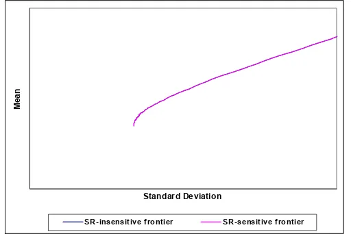
Proposition 2 makes explicit the situations in which there is an SRI cost. The impact of the constraint on the SR ratings depends on the parameterδ1 and on the strength of the constraint. As showed in Proposition 1, ifδ1 >0, resp.δ1 <0, the best SR-rated portfolios are at the top, resp. at the bottom, of the SR-insensitive frontier: by consequence, the SR constraint impacts first the efficient frontier at the bottom, resp. at the top. In addition, the more the investor wants a well-rated portfolio, that is to say the higher the thresholdφ₀, the bigger the portion of the efficient frontier being displaced. In the case where the thresholdφ₀is below the minimum rating of the SR-insensitive frontier, the efficient frontier is even not modified at all. We illustrate the four possible cases through Figures 1 to 4.

In the case where δ1 >0 and 1 0 1

'

' _φ

ι ι

φ ι

> ∑ ∑ − −

(see Figure 1), the SR-sensitive and the

(11)

Figure 1 SR-sensitive frontier versus SR-insensitive frontier with δ1 >0 and 1 0 1

'

' _φ

ι ι

φ ι

> ∑ ∑

− −

Standard Deviation

M

ean

SR-insensitive frontier SR-sensitive frontier

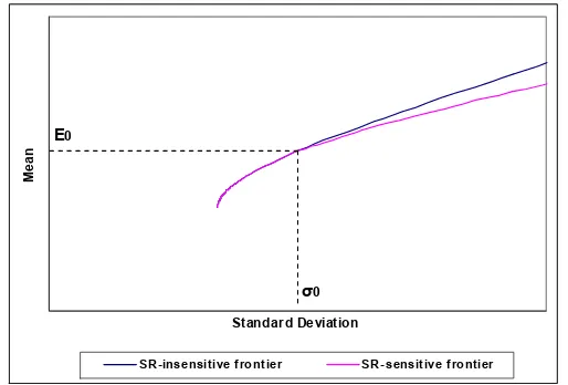
In the case where δ₁ >0 and ₁ ₀

1

'

' _φ

ι ι

φ

ι _<

∑ ∑

− −

(see Figure 2), the sensitive and the

SR-insensitive frontiers are the same above the corner portfolio defined by its expected return

0

E and its expected varianceV₀ =σ₀2. For portfolios with lower expected returns and variances, the SRI constraint induces less efficient portfolios. There is only an SRI cost for investors whose risk aversion parameter is above the thresholdλ₀.

Figure 2 SR-sensitive frontier versus SR-insensitive frontier with δ₁ >0 and ₁ ₀

1

'

' _φ

ι ι

φ

ι _<

∑ ∑

− −

Me

a

n

σ0

(12)

In the case where δ1 <0 and 1 0 1

'

' _φ

ι ι

φ ι

> ∑ ∑ − −

(see Figure 3), the SR-sensitive and the

SR-insensitive frontiers are the same below the corner portfolio(E₀,V₀). For portfolios with higher expected returns and variances, the SRI constraint induces less efficient portfolios. There is only an SRI cost for investors whose risk aversion parameter is below the thresholdλ₀.

Figure 3 SR-sensitive frontier versus SR-insensitive frontier with δ₁ <0 and ₁ ₀

1

'

' _φ

ι ι

φ ι

> ∑ ∑

− −

Mean

σ0

E0

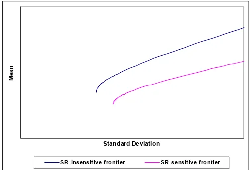
In the case whereδ1 <0 and 1 0 1

'

' _φ

ι ι

φ ι

< ∑ ∑

− −

(see Figure 4), the sensitive and the

(13)

Figure 4 SR-sensitive frontier versus SR-insensitive frontier with δ1 <0 and 1 0 1

'

' _φ

ι ι

φ ι

< ∑ ∑

− −

M

ean

To sum up, while the investor’s risk aversion is generally left out of the story in the SRI practice, we show in this Section that this parameter matters in the cost of responsible investing9. Indeed, we show that this SR cost depends on the link between SR ratings and financial returns and on the investor’s risk aversion; four cases being possible: a) the SR-sensitive frontier is the same as the SR-inSR-sensitive frontier (i.e. no cost), b) only the left portion of the efficient frontier is penalized (i.e. a cost for high-risk-aversion investors only), c) only the right portion of the efficient frontier is penalized (i.e. a cost for low-risk aversion investors only), and d) the full frontier is penalized (i.e. a cost for all the investors).

3) Portfolio selection with a risk-free asset

In this section, we assume the existence of a risk-free asset and we explore, in this case, the impact of considering responsible ratings in the mean-variance portfolio selection. Indeed,

9

(14)

the social responsibility of this risk-free asset should also be taken into account. So, we assess first the social responsibility of the optimal portfolios obtained by an SR-insensitive investor. And then we study whether an SR-sensitive investor is penalized by requiring portfolios with high SR standards.

Denote by rthe return of the risk-free asset and byω_r the fraction of wealth invested in this free asset. The standard mean-variance portfolio selection in the presence of a risk-free asset has been extensively studied by Lintner (1965) and Sharpe (1965). It corresponds to Problem 3.

Problem 3

The investor wants to solve the following program:

{ }

1 '

' 2 '

max

= +

∑ − +

r r

to subject

r

ω ι ω

ω ω λ ω μ ω

ω ₍₅₎

In the mean-standard deviation plan, the set of optimal portfolios is referred as the well-known Capital Market Line (CML). As the investor does not consider responsible ratings in her optimization, we refer it here as “SR-insensitive capital market line”.

(15)

Proposition 3

(i) Along the SR-insensitive capital market line, the responsible rating φ_p is a linear function of the expected returnμ_p:

φ_p δ δ* μ_p the expected return tends to the infinite.)

(iii) Ifδ1*<0, φp ranges from *φ (for the minimum-variance portfolio) to−∞ (when the expected return tends to the infinite).

Proof: see Appendix 3

Proposition 3 attributes an SR rating of any portfolio of the SR-insensitive capital market line. From the optimality conditions comes the fact that, along the capital market line,

both the SR rating φpand the expected returnμp are linear functions of the quantity _λ 1

It is

(16)

where the trade-off appears between risk aversion and SR rating. If * 0

1 >

δ , resp. * 0

1 <

δ , the riskier the optimal portfolio, the better, resp. the worse, its SR rating. In other words, if * 0

1 >

δ , resp. * 0

1 <

δ , the best SR-rated portfolios are at the top, resp. at the bottom, of the SR-insensitive capital market line.

Similarly to Section 2, we now consider the case of SR investors wishing high SR standards and so, requiring the portfolio rating φ_p =ω'φ +ω_rφ* to be above a thresholdφ₀. This corresponds to Problem 4.

Problem 4

The investor wants to solve the following program:

{ }

0

* '

1 '

' 2 '

max

φ φ ω φ ω φ

ω ι ω

ω ω λ ω μ ω

ω

≥ +

= = +

∑ − +

r p

r r

to subject

r

(7)

(17)

Proposition 4

The shape of the SR-sensitive capital market line depends on the sign of * 1

δ and on the threshold valueφ₀ in the following way:

0 capital market line is a hyperbola

lying below the SR-insensitive capital market line. Forλ>λ*₀, the SR-sensitive capital market line is identical to the SR-insensitive capital market

line.

The SR-sensitive capital market line is the same as the SR-insensitive capital market line

0

* φ

φ < The SR-sensitive capital market line differs totally from the SR-insensitive capital market line and

becomes a hyperbola.

Forλ <λ*₀, the SR-sensitive capital market line is identical to the SR-insensitive capital market

line.

For *

0 λ

λ > , the SR-sensitive capital market line is a hyperbola

lying below the SR-insensitive capital market line.

With

(18)

on the parameter * 1

δ and on the strength of the constraint. As showed in Proposition 3, ifδ1* >0, resp. 0

* 1 <

δ , the best SR-rated portfolios are at the top, resp. at the bottom, of the SR-insensitive capital market line: by consequence, the SR constraint impacts first the capital market line at the bottom, resp. at the top. However, contrary to the case without a risk-free asset, the modified part of the capital market line has a different mathematical form: for this segment, the capital market line becomes a hyperbola in the mean-standard deviation plan. Figures 5 to 8 illustrate the four cases.

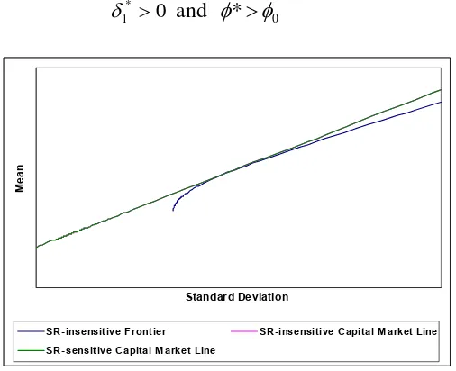
In the case where * 0

1 >

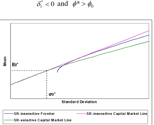
δ and φ*>φ₀ (see Figure 5), the sensitive and the SR-insensitive capital market lines are the same and there is no SRI cost at all. This is the best case.

Figure 5 SR-sensitive capital market line versus SR-insensitive capital market line with

0

* 1 >

δ and φ*>φ₀

Me

a

n

SR-insensitive Frontier SR-insensitive Capital M arket Line SR-sensitive Capital M arket Line

In the case where δ1* >0 and φ*<φ0 (see Figure 6), the sensitive and the

SR-insensitive capital market lines are the same for portfolios below the corner portfolio defined by its expected return *

0

E and the expected variance 2* 0 *

0 =σ

(19)

SR-sensitive capital market line becomes a hyperbola. There is an SRI cost only for investors with cold feet, that is to say with a risk aversion parameter above the thresholdλ*₀.

0

* 1 >

δ and φ*<φ₀

Me

an

E0*

σ0*

In the case where * 0

1 <

δ and φ*>φ₀ (see Figure 7), the sensitive and the SR-insensitive capital market lines are the same for portfolios above the corner portfolio

) ,

(E₀* V₀* . Above this portfolio, the SR-sensitive capital market line becomes a hyperbola. There is an SRI cost only for investors with a risk aversion parameter below the thresholdλ*₀.

0

* 1 <

δ and φ*>φ₀

Me

an

E0*

(20)

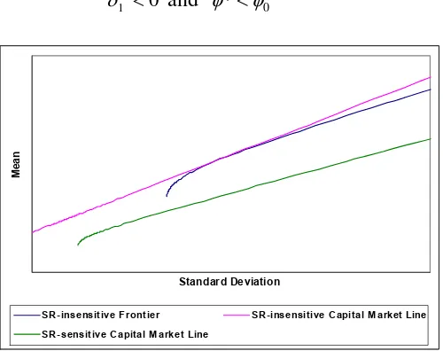
In the case where δ1*<0 and φ*<φ0 (see Figure 8), the sensitive and the

SR-insensitive capital market lines differ entirely. The SR-sensitive capital market line is no longer a line but a hyperbola. This is the most disadvantageous case: there is an SRI cost for all the investors.

0

* 1 <

δ and φ*<φ₀

Me

a

n

(21)

4) Application to an emerging bond portfolio

This section illustrates the results of Sections 2 and 3 by considering the case of a responsible US investor on the emerging bond market.

We consider the EMBI+ indices from JP Morgan as proxy for emerging bond returns. These indices track total returns for actively traded external debt instruments in emerging markets.10 The indices are expressed in US dollars and taken at a monthly frequency from January 1994 to October 2009. They are extracted from Datastream. Descriptive statistics are available in Appendix 5.

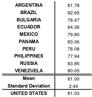
In the same way as Scholtens (2009), we use the Environmental Performance Index (EPI) as responsible ratings. The EPI is provided jointly by the universities of Yale and Columbia in collaboration with the World Economic Forum and the Joint Research Centre of the European Commission. EPI focuses on two overarching environmental objectives: reducing environmental stress to human health and promoting ecosystem vitality and sound management of natural resources. These objectives are gauged using 25 performance indicators tracked in six well-established policy categories, which are then combined to create a final score. EPI scores attributed in 2008 are reported in Table 3.

10

(22)

Table 3 Environmental Performance Index 2008

ARGENTINA 81.78

BRAZIL 82.65

BULGARIA 78.47

ECUADOR 84.36

MEXICO 79.80

PANAMA 83.06

PERU 78.08

PHILIPPINES 77.94

RUSSIA 83.85

VENEZUELA 80.05

Mean 81.00

Standard Deviation 2.44

UNITED STATES 81.03

Sources: Universities of Yale and Columbia.

Here, the portfolio EPI is defined in the same way as in eq. (2). We start by estimating the portfolio EPI along the SR-insensitive frontier, which corresponds to estimating the relationship (3) of Proposition 1. We obtain the following estimates for the parameters δ₀ andδ₁:

00 . 76 ˆ

0 =

δ δˆ₁ =0.30

Asδˆ₁ >0, the portfolio EPI increases with the expected return on the SR-insensitive efficient frontier: a 1%/year increase in expected returns corresponds to an increase of 0.30 in the EPI portfolio. The minimal EPI portfolio on the SR-insensitive frontier is obtained for the

minimum-variance portfolio and is equal to 78.26 ˆ

' ˆ '

1 1

= ∑ ∑ − −

ι ι

φ ι

.

(23)

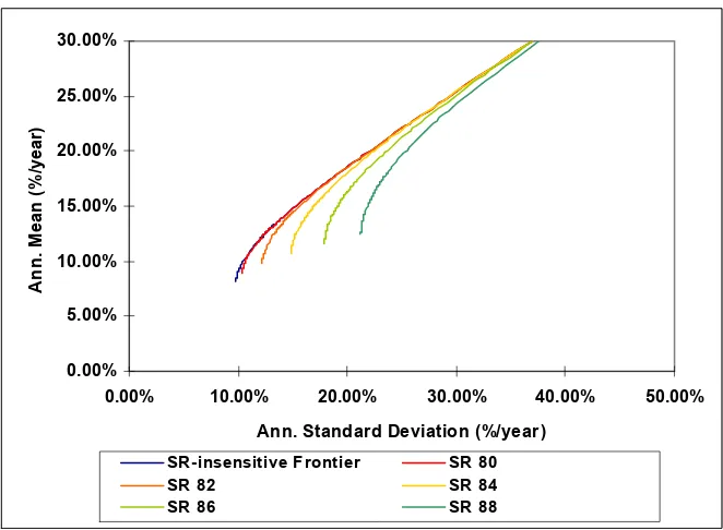
Figure 9 SR-sensitive frontiers versus SR-insensitive frontier for the EMBI+ indices, January 1994 to October 2009

0.00% 5.00% 10.00% 15.00% 20.00% 25.00% 30.00%

0.00% 10.00% 20.00% 30.00% 40.00% 50.00%

Ann. Standard Deviation (%/year)

A

n

. M

ean

(

%

/year

)

SR-insensitive Frontier SR 80

SR 82 SR 84

SR 86 SR 88

Table 4 Corner portfolios for which the SR constraint is binding

0

φ λ₀ Expected return E₀

(%/year)

Expected volatility σ₀ (%/year)

82 3.14 20.13 22.22

84 2.05 26.84 32.17

86 1.52 33.55 42.48

(24)

As expected from Proposition 2, for 78.26 ˆ

' ˆ '

1 1

0 =

∑ ∑ < −₋

ι ι

φ ι

φ , the SR-sensitive frontier is the

same as the SR-insensitive frontier. For 78.26 ˆ

' ˆ '

1 1

0 =

∑ ∑ >

− −

ι ι

φ ι

φ , the SR-sensitive frontier differs

from the SR-insensitive frontier at the bottom and is the same at the top. For instance, with a threshold equal to 84 on the portfolio EPI, the SR-sensitive and the SR-insensitive frontiers are the same for expected returns above 26.84%/year and differ for expected returns below 26.84%/year. In the case of emerging bonds, improving the portfolio EPI costs more for investors with high risk aversion.

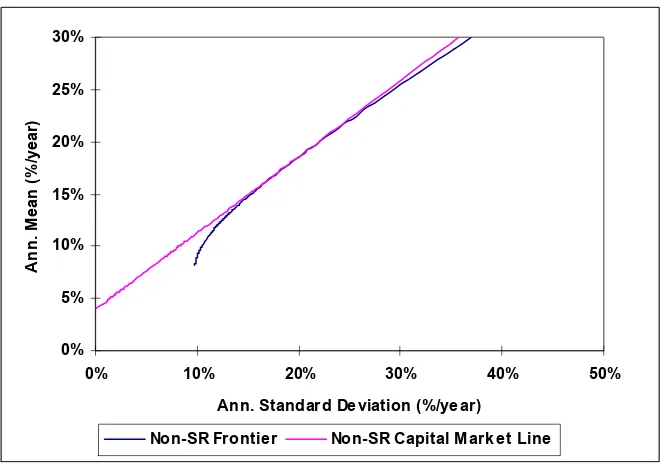
In order to illustrate Problems 3 and 4, we rely on the US 1-month interbank rate as a risk-free asset.11 Its responsible rating corresponds to the EPI of the United Statesφ*=81.03. Then, we estimate the parameters δ₀* andδ₁*:

95 . 80 ˆ*

0 =

δ δˆ₁* =0.02

As ˆ* 0

1 >

(25)

Figure10 SR-insensitive capital market line for the EMBI+ indices, January 1994 to October 2009

0% 5% 10% 15% 20% 25% 30%

0% 10% 20% 30% 40% 50%

A

n

. Mean

(

%

/year

)

Non-SR Frontier Non-SR Capital Market Line

(26)

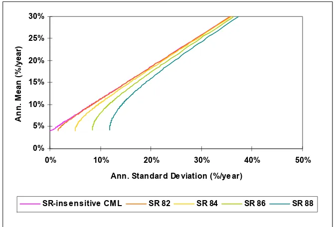
Figure 11 SR-sensitive capital market lines versus SR-insensitive capital market lines for the EMBI+ indices, January 1994 to October 2009

0% 5% 10% 15% 20% 25% 30%

0% 10% 20% 30% 40% 50%

A

n

. Mean

(

%

/year

)

SR-insensitive CML SR 82 SR 84 SR 86 SR 88

Table 5 Corner portfolios for which the SR constraint is binding

0

φ λ₀ Expected return E₀

(%/year)

Expected volatility σ₀* (%/year)

82 1.16 50.01 63.06

84 0.38 144.97 193.08

86 0.23 239.93 323.11

88 0.16 334.89 453.13

(27)

particularly low sensitivity * 1

ˆ

δ . For example, if we consider a thresholdφ₀ =82, the corner portfolio has an expected return of 50.01%/year and an expected volatility of 63.06%/year, meaning that for expected returns below 50.01%/year, the SR-sensitive and SR-insensitive capital market lines are disconnected. However, we observe in Figure 11 that the SR-insensitive and SR-sensitive capital market lines are very close for expected returns slightly below 50.01%/year.

This numerical application highlights that the cost implied by high environmental requirements in an emerging bond portfolio differs according to the investor’s risk aversion. In this particular case, it costs more to be green for investors with cold feet. Let us now focus on a typical investor. Sharpe (2007) suggests that the “representative investor” has a risk aversion parameter

7 . 0

2 =

λ in the traditional mean-variance optimization of eq. (1). We seek

(28)

Figure 12 Displaced optimal portfolios for the “representative investor”

0.00% 5.00% 10.00% 15.00% 20.00% 25.00% 30.00%

0.00% 10.00% 20.00% 30.00% 40.00% 50.00%

A

n

. M

ean

(

%

/year

)

SR-insensitive Frontier SR 82

SR 84 SR 86

SR 88 SR 90

For the “representative investor”, the constraint on the portfolio EPI has no cost while the threshold is below 82.37, which is slightly above the average EPI rating of the sample’s countries. When the threshold is above 82.37, an SRI cost appears and the optimal portfolio is no longer on the SR-insensitive frontier. This SRI cost rises with the strength of the constraint. In this case, the “representative investor” is directly concerned by the disconnect between SR-sensitive and SR-insensitive frontiers for reasonable SR thresholds.

5) Conclusion

(29)

debate, our paper aimed at modelling SRI in the traditional mean-variance portfolio selection framework (Markowitz, 1952).

In our study, SRI is introduced in the mean-variance optimization as a constraint on the average responsible rating of the underlying entities. Our results are detailed so that they are ready to use by practitioners. Indeed, we show that a threshold on the responsible rating may impact the efficient frontier in four different ways, depending on the link between the returns and the responsible ratings and on the strength of the constraint. The SR-sensitive efficient frontier can be: a) identical to the SR-insensitive efficient frontier (i.e. no cost at all), b) penalized at the bottom only (i.e. a cost for high risk-aversion investors only), c) penalized at the top only (i.e. a cost for low risk-aversion investors only), d) totally different from the SR-insensitive efficient frontier (i.e. a cost for every investor). In other words, if portfolio ratings increase (resp. decreases) with the expected return along the traditional efficient frontier, the SRI cost arises first at the bottom (resp. at the top) of the frontier. The results are the same in the presence of a risk-free asset. Our work highlights the fact that the investor’s risk aversion clearly matters in the potential cost of investing responsibly, this cost being zero in some cases. We strongly believe that this finding could help portfolio managers of SRI funds.

(30)

REFERENCES

Barracchini, C., 2007. An ethical investments evaluation for portfolio selection., Journal of Business Ethics and Organization Studies 9, 1239-2685.

Basak, G., Jagannathan, R., Sun, G., 2002. A direct test of mean-variance efficiency of a portfolio. Journal of Economic Dynamics and Control 26, 1195-1215.

Beal, D., Goyen, M., Philips, P., 2005. Why do we invest ethically? Journal of Investing 14, 66-77.

Best, M., Grauer, R., 1990. The efficient set mathematics when mean-variance problems are subject to general linear constraints. Journal of Economics and Business 42, 105-120.

de Roon, F., Nijman T., 2001. Testing for mean-variance spanning: a survey. Journal of Empirical Finance 8, 111-156.

Dorfleitner, G., Leidl, M., Reeder J., 2009. Theory of social returns in portfolio choice with application to microfinance. Working Paper, University of Regensburg.

Drut, B., 2009. Nice guys with cold feet: the cost of responsible investing in the bond markets”, Working Paper No 09-34, Centre Emile Bernheim, Université Libre de Bruxelles. European Sustainable Investment Forum, 2008. European SRI Study. European Sustainable Investment Forum, Paris. Available at: http://www.eurosif.org/publications/sri_studies . Farmen, T., Van Der Wijst, N., 2005. A cautionary note on the pricing of ethics. Journal of Investing 14, 53-56.

Geczy, C., Stambaugh, R., Levin, D., 2006. Investing in socially responsible mutual funds. Working Paper, Wharton School of the University of Pennsylvania.

Landier, A., Nair V., 2009. Investing For Change. Oxford University Press, Oxford.

Lintner, J., 1965. The valuation of risky assets and the selection of risky investment in stock portfolios and capital budgets. Review of Economics and Statistics 47, 13-37.

Lo, A., 2008. Hedge Funds: An Analytic Perspective. Princeton University Press, Princeton. Markowitz, H., 1952. Portfolio selection., Journal of Finance 7, 77-91.

Principles for Responsible Investment, 2009. PRI Annual Report. Principles for Responsible Investment, New York. Available at:

http://www.unpri.org/files/PRI%20Annual%20Report%2009.pdf .

(31)

Social Investment Forum, 2007. Report on socially responsible investing trends in the United States. Available at:

http://www.socialinvest.org/resources/pubs/documents/FINALExecSummary_2007_SIF_Tre nds_wlinks.pdf .

Sharpe, W., 1965. Capital asset prices: a theory of market equilibrium under conditions of risk. Journal of Finance 19, 425-442.

Sharpe, W., 2007. Expected utility asset allocation, Financial Analysts Journal 63, 18-30. Steinbach, M., 2001. Markowitz revisited: mean-variance models in financial portfolio analysis. Society for Industrial and Applied Mathematics Review 43, 31-85.

Appendix 1

Following Best and Grauer (1990), in the standard mean-variance case, the weights vector that solves the problem is:

⎥

The corresponding expected return μPstands as:

⎥⎦

And the expected variance 2

P

The corresponding responsible rating φPis also a linear function of_λ 1

As the expected return is also a linear function of

λ

1

, it is possible to express the responsible rating as a linear function of the expected return:

(32)

2

Appendix 2

The mean-variance optimization with the linear constraint on the portfolio rating has the same portfolio solutions as the standard mean-variance optimization, while the constraint is not binding. This is verified if the portfolio rating of the efficient portfolio from the traditional mean-variance optimization is above the threshold φ₀. Two cases have to be distinguished: where δ₁ >0 and where δ₁ <0.

Case δ₁ >0

In this case, the portfolio rating increases linearly with the expected return in the traditional mean-variance optimization. The minimal portfolio rating is

ι constraint on the portfolio rating is inactive and the solutions are the same as in the traditional mean-variance optimization. If ₁ ₀

1

, the constraint on the portfolio rating is binding at the bottom of the efficient frontier and inactive at the top. Indeed, the constraint is binding for λ >λ₀with:

In the mean-variance plan, this corner portfolio is the one for which the portfolio rating isφ₀.

To compute the portion of the efficient frontier for which the linear constraint on the portfolio rating is binding, we apply the results of Best and Grauer (1990):

(33)

1

In this case, the portfolio rating decreases linearly with the expected return in the traditional mean-variance optimization. The maximal portfolio rating is

ι

constraint on the portfolio rating is binding. If ₁ ₀

1

, the constraint on the portfolio rating is binding at the top of the efficient frontier and inactive at the bottom. Indeed, the constraint is binding forλ <λ₀.

The equation of the portion of the efficient frontier for which the constraint is binding is the same as for the case δ1 >0.

Appendix 3

Following Best and Grauer (1990), in the traditional mean-variance case, the portfolio solutions stand as:

[

( )

]

(34)

[

( )' ( )

]

The responsible rating of the efficient portfolios is a linear function of

λ

, it is possible to express the responsible rating φ_P of the efficient portfolios as a linear function of the expected returnμ_P:

[

( * )' ( )

]

Appendix 4

The mean-variance optimization with the linear constraint on the portfolio rating has the same portfolio solutions as the standard mean-variance optimization while the constraint is not binding. This is verified if the portfolio rating of the efficient portfolio from the traditional mean-variance optimization is above the thresholdφ₀. Two cases have to be distinguished: where δ1* >0 and where 0

* 1 <

δ .

Case δ1* >0

(35)

Indeed, the constraint is binding for λ >λ*₀with:

The risk aversion parameter λ*₀corresponds to the portfolio with the expected return: )

And the expected variance:

)

To compute the portion of the efficient frontier for which the linear constraint on the portfolio rating is binding, we apply the results of Best and Grauer (1990):

)

Indeed, when the constraint on the portfolio rating is binding, the Capital Market Line is no longer a linear function in the mean-standard deviation plan but a hyperbola.

Case δ₁* <0

In this case, the portfolio rating φ_pdecreases linearly with the expected return μ_pin the traditional mean-variance optimization. The maximum portfolio rating is *φ . If φ*<φ₀, the constraint on the portfolio rating is always active: the entire Capital Market Line becomes a hyperbola in the mean-standard deviation plan. If φ*>φ₀, the constraint on the portfolio rating is binding at the top of the Capital Market Line. The modification of the Capital Market Line occurs for the same risk aversion parameter *

0

λ as for the case * 0

1 >

(36)

Appendix 5 Descriptive statistics for the EMBI + indices in US dollars, January 1994 to October 2009

Ann. MeanAnn. Std. Dev.

Sharpe

Ratio Skewness Kurtosis Maximum Minimum

ARGENTINA 4.94% 28.84% 0.03 -1.07 9.37 33.80% -43.90%

BRAZIL 15.03% 21.40% 0.51 -0.62 8.22 26.47% -27.17%

BULGARIA 15.10% 20.26% 0.55 -0.98 13.96 25.77% -36.38%

ECUADOR 16.19% 33.51% 0.36 -1.47 10.10 28.29% -55.78%