J. Phys. A: Math. Gen.38(2005) L759–L768 doi:10.1088/0305-4470/38/45/L03
LETTER TO THE EDITOR
A formula to compute the microcanonical volume of
reactive initial conditions in transition state theory
H Waalkens, A Burbanks1and S Wiggins
School of Mathematics, Bristol University, University Walk, Bristol, BS8 1TW, UK E-mail:[email protected]
Received 6 September 2005, in final form 5 October 2005 Published 26 October 2005
Online atstacks.iop.org/JPhysA/38/L759
Abstract
We present the formal proof of a procedure to compute the phase-space volume of initial conditions for trajectories that, for a constant energy, escape or ‘react’ from a multi-dimensional potential well with one or several exit/entrance channels. The procedure relies on a phase-space formulation of transition state theory. It gives the volume of reactive initial conditions as the sum over the exit/entrance channels where each channel contributes by the product of the phase-space flux associated with the channel and the mean residence time in the well of those trajectories which escape through the channel. An example is given to demonstrate the computational efficiency of the procedure.
PACS numbers: 45.20.Jj, 05.45.−a, 34.10.+x, 82.20.Db
(Some figures in this article are in colour only in the electronic version)
1. Introduction
The problem of escape from a potential well where exit from the well is possible through channels that are associated with saddle points is a common problem in many areas of physics. In this letter, we prove a formula and present a procedure based on the formula that enables one to compute the phase-space volumes of initial conditions in the well that, for a fixed energy, lead to trajectories which escape from the potential well through any of these channels. We note that a similar result, the classical limit of the so-calledspectral theorem, has been obtained by Pollak [1] in the context of molecular collisions (the spectral theorem relates time delays in collisions to the density of states; see [2] for the historical background). The implementation of our procedure relies on the recent development of aphase-spaceformulation of transition state theory based on general ideas from dynamical systems theory [3–8] and we therefore find it useful to provide a formal proof of the spectral theorem especially in this context.
1 Present address: Department of Mathematics, University of Portsmouth, Lion Terrace, Portsmouth, P01 3HE, UK.
For energies slightly above the saddle, phase-space transition state theory, which is algorithmic in nature, solves the key problem of how to define and construct a dividing surface near a saddle point, which locally divides the energy surface into two disjoint components and which is free of local ‘recrossing’. These properties which are essential for rate computations will also play an important role in what follows.
In recent years, transition state theory has been recognized as a very fruitful approach whose applicability goes far beyond its origin of conception in chemistry. It has been used e.g. in atomic physics [9], studies of the rearrangements of clusters [10], solid state and semi-conductor physics [11,12], cosmology [13] and celestial mechanics [14]. The results presented in this letter are of central interest for all of these areas as they open the way to study fundamental questions like the violation of ergodicity assumptions on the dynamics which are typically made in statistical approaches like Rice–Ramsperger–Kassel–Marcus (RRKM) theory [15].
Before we derive the formula for the volume of reactive initial conditions in a potential well, we recapitulate the building blocks of phase-space transition state theory.
2. Phase-space transition state theory
We start with an equilibrium point for Hamilton’s equations which is of saddle-centre–centre type (which we refer to as ‘saddle’ for short, in what follows). A detailed theory for phase-space transport associated with saddles has been developed in recent years [3–8]. For energies slightly above that of a saddle, on each(2n−1)-dimensional energy surface withnbeing the number of degrees of freedom, there exists an invariant(2n−3)-dimensional sphereS2n−3of saddle stability type, which is significant for two reasons:
• It is the ‘equator’ of a particular (2n−2)-dimensional sphere, which we take as the
dividing surface. The equator separates the dividing surface into two hemispheres which have the structure of open(2n−2)-dimensional balls. Except for the equator (which is an invariant manifold), the dividing surface is locally a ‘surface of no return’ in the sense that trajectories which have crossed the dividing surface must leave a certain neighbourhood of the dividing surface before they can possibly cross it again. For energies ‘sufficiently close’ to the energy of the saddle, the dividing surface satisfies thebottleneck property. This means that the energy surface has locallythe geometrical structure of S2n−2×I (i.e.,(2n−2)-sphere×interval where the interval corresponds to a so-called
reaction coordinate) and the dividing surface divides the energy surface into two disjoint components. Moreover, theonlyway a trajectory can pass from one component of the energy surface to the other in the ‘forward’ direction is through one hemisphere and the only way to pass in the ‘backward’ direction is through the other hemisphere. The hemispheres are thus the gateways to the exit and entrance channels for the energy surface components. The fluxes through the forward and backward hemispheres are of equal magnitude and opposite sign so that the total flux through the dividing surface is zero. However, for our particular choice of dividing surface, thedirectionalflux through each hemisphere is minimal in a sense made precise in [16].
significance is that the only way that trajectories can pass through the dividing surface is if they are inside a particular region of the energy surface enclosed by the stable and unstable spherical cylinders.
For a system with two degrees of freedom, the NHIM is a periodic orbit. If this system is of type ‘kinetic-plus-potential’ the configuration space projection of the periodic orbit connects, for an energy slightly above the energy of the potential saddle, two branches of an iso-potential line and this is the basis for the construction of the so-calledperiodic orbit dividing surface
(PODS) in the seminal work by McLafferty, Pechukas and Pollak [17–20].
For higher dimensions, the phase-space structures mentioned above can be computed via a procedure based on Poincar´e–Birkhoff normalization [7, 8] which yields a nonlinear symplectic transformation of the original phase-space coordinates to new coordinates referred to as the normal form coordinates. The NHIM, the local parts of its stable and unstable manifolds and the dividing surface are simply given as normal form coordinate hyperplanes. The phase-space structures are then mapped into the original phase-space coordinate system by the inverse of the normal form transformation.
The phase-space structures, and techniques, are the key to analysing the problem of ‘escape’ or ‘reaction’ from a phase-space region. However, in order to use them, we must first derive a more general result.
3. A rigorous statement on volumes within the energy surface that are ‘swept out’ by trajectories
Let us consider an n degree-of-freedom Hamiltonian system (M, ω) where M is a
(2n)-dimensional manifold (the phase space) andωis a symplectic 2-form. The Hamiltonian function, which is assumed not to depend on time, isH. The volume of aphase-space region
is obtained by integrating over it the(2n)-form=ωn/n!. Since energy is conserved under
the dynamics, it makes sense to consider the volumes of regions in a single energy surface E. A differential formηto measureenergy surface volumeis a(2n−1)-form by which the
phase-space volume formcan be decomposed according to=dH∧η[21].
We want to derive a rigorous statement about how the integration ofηover energy surface regions swept out by trajectories can be evaluated. The statement is phrased in a way that makes it directly applicable to the setting of transition state theory elucidated above.
Theorem 1. Let S and S′ be two (2n−1)-dimensional manifolds in M with S being a
coordinate hyperplane q1 = 0 of a canonical coordinate system (p1, . . . , pn, q1, . . . , qn).
Moreover, assumeq˙1>0in S which implies that S is transverse to the Hamiltonian flow.S′is
arbitrary and may coincide with S. Let E be a regular value of H andEbe the corresponding
energy surface. Assume thatB⊂S∩Eis a(2n−2)-dimensional manifold which, under the
map induced by the Hamiltonian flow, has a continuous imageB′inS′∩
E. Assume that the
corresponding orbit segments start on B and end onB′without having further intersections
with B orB′. Then the energy surface volume of the set M
B→B′, swept out by the orbit
segments between B andB′, is given by
vol(MB→B′)=φBtB, (1)
with
φB =
B ′,
′= ω n−1
(n−1)!
C
C’
S Γ
Figure 1. Sketch of a(2n−1)-dimensional manifoldSand a two-dimensional closed manifold
Cin the(2n)-dimensional phase space. The deformation ofCconsists ofC′, which is the image ofCinSunder the inverse Hamiltonian flow, andŴ, which is swept over by letting the inverse Hamiltonian flow act on the boundary∂C.
being the flux through B, and with
tB =
Bt ′
B′
, (3)
being the average of the passage timet :B →R+, which maps points in B to the times they require to reachS′under the Hamiltonian flow.
We start the proof of theorem1 by the following generalization of a result by Binney, Gerhard and Hut [22]
Lemma 2. Given the setting of theorem 1, there exists a sufficiently small phase-space neighbourhood of MB→B′ in which we can construct the canonical coordinates
(H, P2, . . . , Pn, t, Q2, . . . , Qn) which are defined as follows. For a phase-space point in
this neighbourhood, H is the energy at this point,P2, . . . , Pn, Q2, . . . , Qnare the coordinates (p2, . . . , pn, q2, . . . , qn)of the image of this point in S under the inverse flow and t is the time
it takes the point to reach S under the inverse flow.
We first prove this result.
Proof(lemma2). Since the Jacobian of the transformation(p1, p2, . . . , pn, q2, . . . , qn)→ (H, p2, . . . , pn, q2, . . . , qn)which replacesp1byHhas determinant ˙q1, and by our assumption
˙
q1 > 0 inS, it follows that(H, p2, . . . , pn, q2, . . . , qn)are well-defined coordinates in S.
Moreover, from the uniqueness of solutions of ODEs (Hamilton’s equations in this case), it follows that a point in the volume swept out by letting the Hamiltonian flow act onSis uniquely determined by the coordinates(H, p2, . . . , pn, t, q2, . . . , qn)wheretis the time it takes the
inverse flow to map the point back toS.
We now have to show that these coordinates are canonical, i.e. defining ˜ω=dH ∧ dt+
n
k=2 dPk∧ dQk we have to show that, in the above neighbourhood, ˜ω = ω. We thus
For a point inŴ, we choose two basis vectorsu andv for the tangent space of Ŵ at this point. SinceŴis foliated by orbits we can chooseuto be the Hamiltonian vector field at the point under consideration, i.e.u=(p,˙ q)˙ . The vectorvis obtained as the derivative of some phase-space curve(p(λ), q(λ)) which passes through this point, i.e.v = (dp/dλ,dq/dλ). First we applyωto(u, v). This gives
ω(u, v)= n
k=1
((dpk(u)dqk(v)−dpk(v)dqk(u))
= − n
k=1
((∂H /∂qk)(dqk/dλ)+(∂H /∂pk)(dpk/dλ))
= −dH /dλ,
where the last equality follows from the chain rule. Next we apply ˜ωto(u, v). This gives
˜
ω(u, v)=dH (u)dt (v)−dH (v)dt (u)+
n
k=2
(dPk(u)dQk(v)−dPk(v)dQk(u)).
Since H, and Pk and Qk, k = 2, . . . , n, are conserved along trajectories with initial
conditions inS, it follows that dH (u) = dPk(u) = dQk(u) = 0, k = 2, . . . , n. Hence,
˜
ω(u, v) = −dH (v)dt (u), and using dH (v) = dH /dλand dt (u) =1 we see that ˜ω(u, v)
agrees withω(u, v)computed above.
Having proven the generalization of the result by Binney, Gerhard and Hut, we are now in a position to prove formula (1).
Proof(theorem1).Recall that the energy surface volume formηis a(2n−1)-form defined by =dH∧ηwith=ωn/n!. The volume ofM
B→B′is defined by vol(MB→B′)=
MB→B′η.
According to the above, we haveω = ω˜ in a neighbourhood of MB→B′. It follows that
= dH ∧ dt ∧ dP2∧ dQ2 ∧ · · · ∧ dPn∧ dQn from which we can read off η to be η=dt∧dP2∧dQ2∧· · ·∧dPn∧dQn. Carrying out the integration in the direction of the flow,
we get vol(MB→B′)=
BtdP2∧dQ2∧· · ·∧dPn∧dQnwheret (E, P2, . . . , Pn, Q2, . . . , Qn)
is the time it takes the respective point inBto reachS′under the Hamiltonian flow. Since, in
Bwe haveq1=0, andPk=pkandQk =qk, k =2, . . . , n, it follows that the restriction of
dP2∧ dQ2∧ · · · ∧ dPn∧ dQntoBcoincides with the restriction of′=ωn−1/(n−1)! to
B. We thus have vol(MB→B′)= Bt
′where, for a point inB, tis the time to reach its image
inB′under the Hamiltonian flow.
As shown by MacKay [21],′is the(2n−2)-form to measure flux through co-dimension 1 submanifolds of non-critical energy surfaces. Since we assume the energy E under consideration to be non-critical, we can rewrite vol(MB→B′) according to vol(MB→B′) =
φBtBwhereφB =
B
′is the flux through
BandtB =Bt ′B′is the mean passage
time fromBtoB′.
4. Application to an example system
In order to illustrate how theorem1 can be used to analyse the escape or reaction from a potential well, we apply it to the M¨uller–Brown potential energy surface [23,24] which is a frequently used benchmark system in chemistry for testing algorithms in transition state theory (see e.g. [25–27]). The Hamiltonian function for this system is
-1 -0.5 0 0.5 1 x
-0.5 0 0.5 1 1.5 2
y
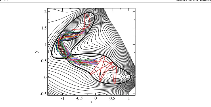
Figure 2. Iso-potential contours for the M¨uller–Brown surface. The bold contour is for energy
E=3 above the saddle at(x, y)≈(−0.822 00,0.624 31). Shown also are local parts of the stable and unstable manifolds of the NHIM (a periodic orbit) and a segment of a trajectory that passes between the wells.
with the potential energy surface
V (x, y)= 4
k=1 Akexp
ak
x−xk0 2+bk
x−xk0 y−yk0 +ck
y−yk0 2, (5)
where
A=(−200,−100,−170,15), a =(−1,−1,−6.5,0.7), b=(0,0,11,0.6), c=(−10,−10,−6.5,0.7), x0=(1,0,−0.5,−1), y0=(0,0.5,1.5,1).
(6)
Equipotentials for this surface are shown in figure 2. The surface has two wells: a deep well at the top and a shallow well with two local minima at the bottom. We want to use formula (1) to compute the volume of initial conditions in either potential well which for a fixed energy slightly above the energy of the saddle at(x, y) ≈ (−0.822 00,0.624 31)can escape to the other well. In phase space, the two wells are separated by a dividing surface which we construct from the Poincar´e–Birkhoff normalization procedure mentioned above. In a phase-space neighbourhood of the corresponding equilibrium point (px, py, x, y) ≈ (0,0,−0.822 00,0.624 31)of Hamilton’s equations this yields a nonlinear transformation of (px, py, x, y)to normal form coordinates(p1, p2, q1, q2). For the present system, which has two degrees of freedom, the dividing surface is a two-dimensional sphere that is given by the intersection of the normal form coordinate hyperplaneq1=0 with the energy surfaceEof
the energyEunder consideration [7].2The NHIM is an unstable periodic orbit; the Lyapunov orbit associated with the saddle. It separates the dividing surface into two hemispheres which are two-dimensional balls or discs. Everytrajectory which passes from the top well to the bottom well has to cross one hemisphere. Everytrajectory which passes from the bottom well to the top well has to cross the other hemisphere. These trajectories are enclosed by the stable and unstable manifolds of the NHIM which have the structure of cylinders whose configuration space projections are shown in figure2.
2 Note that in the present letter, we have adopted a convention for the normal form coordinates that is slightly different
-0.6 -0.4 -0.2 0 0.2 0.4 0.6
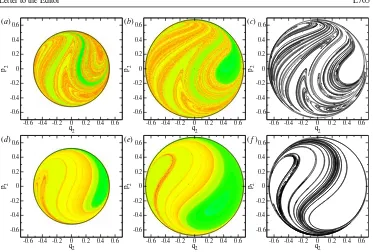
Figure 3. Contours of the residence times on the dividing surface hemispheres. The top (bottom) panels show the dividing surface hemisphere which corresponds to entrance to the lower (top) potential well of the M¨uller–Brown potential. The colours represent the residence times that trajectories started at the corresponding initial condition on the hemisphere spend in the corresponding well. The time increases from green to yellow to red on a standard hue scale. (a) and(d)are for energy E=3 above the saddle energy, (b) and (e) are for energy E=5 above the saddle energy. (c) and(f )show the intersection of the stable manifolds of the NHIM with the corresponding hemisphere for energy E=5 above the saddle energy.
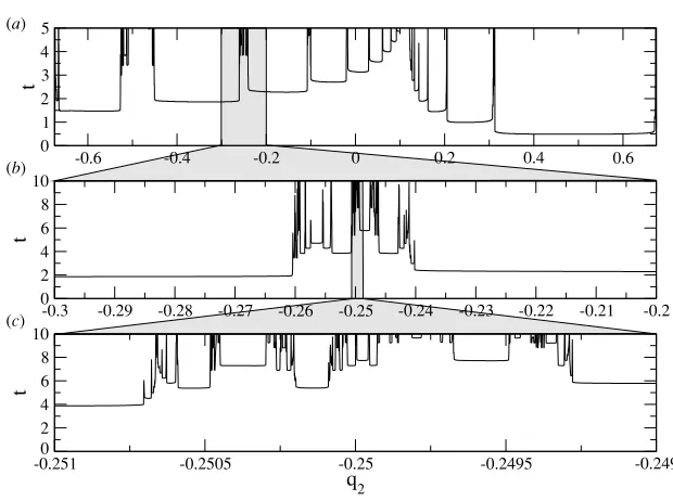
As a consequence of Liouville’s theorem on the conservation of phase-space volume [28], every trajectory (up to a set of measure zero) that enters a well through one hemisphere has to leave it at a later point in time through the other hemisphere. The reactive volume of either well is thus given by the volume swept out by trajectory segments with initial conditions on the corresponding hemisphere and endpoint on the other hemisphere. The NHIM’s stable and unstable manifolds partition the reactive regions into subregions that correspond to different types of reactive trajectories (see [29,30] for a more detailed discussion). This is illustrated in figure3which shows the dividing surface hemispheres for energies E=3 and E=5 above the energy of the saddle. We parameterize the dividing surface hemispheres by the normal form coordinates(q2, p2), and show the contours of the residence time (the time spent in the relevant well before the first exit of the well) for trajectories with initial conditions on these hemispheres. The residence times vary smoothly within the stripes and tongue-shaped patches appearing in figure3. The boundaries of the patches correspond to the intersections of the hemispheres with the stable manifolds of the NHIM which are also shown in figure3. The residence time is infinite on the boundaries. However, the divergence of the residence times is only mild. Upon approaching a boundary from the interior of a single patch the residence time diverges logarithmically. This is illustrated in figure4which shows a one-dimensional cut through one of the hemispheres in figure3. The plateaus of the residence times in figure4
-0.6 -0.4 -0.2 0 0.2 0.4 0.6 0
1 2 3 4 5
t
-0.3 -0.29 -0.28 -0.27 -0.26 -0.25 -0.24 -0.23 -0.22 -0.21 -0.2 0
2 4 6 8 10
t
-0.251 -0.2505 -0.25 -0.2495 -0.249
q2
0 2 4 6 8 10
t
(a)
(b)
(c)
Figure 4.(a) Distribution of residence times along the linep2=0 in figure3(e). (b) and (c) show
successive magnifications of a part of the graph in (a).
singularities form a self-similar structure which is well known from scattering theory. For a more detailed discussion of these structures, see [30].
Theorem1at first only applies to regions in the interior of the patches in figure3. Utilizing standard arguments from integration theory it follows from the fact that the reactive volume of a well is finite that the integrals in equations (2) and (3) can be extended over a whole patch and also that the summation over the infinite number of patches converges. The summation over the patches gives the reactive volumes of a well as the product of the flux and the average total of the residence times of trajectories with initial conditions on the corresponding dividing surface hemisphere. In the case of two degrees of freedom where the NHIM is a periodic orbit, the flux is simply given by the action of the periodic orbit. For systems with more degrees of freedom the flux is given by a generalized action integral over the NHIM which is easily computed from the normal form [16]. The average residence time can be efficiently computed from a Monte Carlo integration [29,30].
We apply the above procedure for energies E = 3 and E = 5 above the
saddle and compare the results with a computationally expensive brute-force calculation in which we sample initial conditions (uniformly distributed with respect to the measure δ(E−H )dxdydpxdpy) on the entire energy surface components associated with the potential
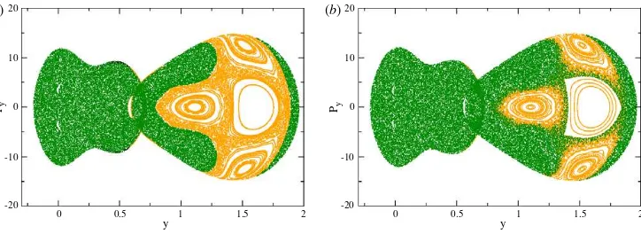
wells and integrate them in time until they either escape or reach a large cut-off time after which escape is very unlikely. Figure5shows the resulting survival probabilitiesP (t ), i.e. the normalized histogram of trajectories which stay in the well under consideration up to timet. The functionsP (t )saturate for largetat valuesP∞where 1−P∞can be identified with the quotient of the reactive volume of a well and the total energy surface volume of that well. For each well, and for both studied energies,P∞isnotequal to zero, indicating that the motions in the wells are not ergodic. This is further illustrated in figure6which shows the dynamics in terms of surfaces of section with the section conditionpx =0,p˙x >0. The ‘bottleneck’
(a)
E = 3
∆
E = 5
∆
0 1000 2000 3000 4000 5000
t
Figure 5. Survival probabilities for trajectories with initial conditions in the top well (a) and bottom well (b) of the M¨uller–Brown potential for energies E =3 and E =5 above the saddle. The inset in (a) shows a magnification of the survival probability graph for E=3. (a)20
E = 5 (b) above the saddle. Green dots mark reactive trajectories; orange dots mark non-reactive trajectories. The region to the left (right) ofy≈0.624 31 corresponds to the bottom (top) well of the M¨uller–Brown potential in figure2.
y ≈ 0.624 31). The parts to the left and right ofy ≈ 0.624 31 in figure6 correspond to the bottom and top wells of the M¨uller–Brown potential, respectively. Reactive trajectories and non-reactive trajectories are marked green and orange, respectively. In agreement with the survival probability curves in figure5, the surfaces of section in figure6indicate that the portion of reactive trajectories is much higher in the lower well than it is in the top well. It is worth mentioning that knowledge of the area of a region in the surface of section (occupied e.g. by reactive or non-reactive trajectories) alone is not sufficient to compute the volume of the corresponding three-dimensional region on the energy surface (see [22] for a thorough discussion of this issue).
For comparison, figure5also shows the values for the reactive volume computed from formula (1) as horizontal lines. In each case the computation of P∞ using (1) is able to reproduce the results from the brute-force method with an error less than 2%.
5. Conclusions and outlook
energy surface to a(2n−2)-dimensional integral over a dividing surface hemisphere which has a much simpler parametrization than the energy surface. As indicated in the example shown it opens the way to study fundamental questions in the context of the transition state theory, such as non-RRKM behaviour and memory effects. If several exit/entrance channels coexist, one has to apply the scheme illustrated in the example to each channel individually and sum over the resulting terms (1). The method has no limitations concerning the number of degrees of freedom nor on the type of Hamiltonian, which may have magnetic or Coriolis terms. For high-dimensional systems, the flux is also computed easily from the normal form [16]. Similarly, the mean passage time associated with an entrance channel can be obtained very efficiently from a Monte Carlo integration as we already demonstrated in applications to high-dimensional systems in celestial mechanics and chemistry [29, 30] for which we computed the phase-space structures mentioned earlier [8,31].
Acknowledgments
We are grateful to A Biternas for providing us with the data that lead to the surfaces of section in figure6. This work was supported by the Office of Naval Research, EPSRC and the Royal Society.
References
[1] Pollak E 1981J. Chem. Phys.746763
[2] Brumer P, Fitz D E and Wardlaw D 1980J. Chem. Phys.70386 [3] Wiggins S 1990PhysicaD44471
[4] Wiggins S 1992Chaotic Transport in Dynamical Systems(Berlin: Springer)
[5] Wiggins S 1994Normally Hyperbolic Invariant Manifolds in Dynamical Systems(Berlin: Springer) [6] Wiggins S, Wiesenfeld L, Jaff´e C and Uzer T 2001Phys. Rev. Lett.865478
[7] Uzer T, Jaff´e C, Palaci`an J, Yanguas P and Wiggins S 2002Nonlinearity15957 [8] Waalkens H, Burbanks A and Wiggins S 2004J. Chem. Phys.1216207 [9] Jaff´e C, Farrelly D and Uzer T 2000Phys. Rev. Lett.84610
[10] Komatsuzaki T and Berry R S 1999J. Chem. Phys.1109160
[11] Jacucci G, Toller M, DeLorenzi G and Flynn C P 1984Phys. Rev. Lett.52295 [12] Eckhardt B 1995J. Phys. A: Math. Gen.283469
[13] de Oliveira H P, Ozorio de Almeida A M, Damia o Soares I and Tonini E V 2002Phys. Rev.D65083511 [14] Jaff´e C, Ross S D, Lo M W, Marsden J, Farrelly D and Uzer T 2002Phys. Rev. Lett.89011101
[15] Steinfeld J I, Francisco J S and Hase W L 1989Chemical Kinetics and Dynamics(Englewood Cliffs, NJ: Prentice Hall)
[16] Waalkens H and Wiggins S 2004J. Phys. A: Math. Gen.37L435 [17] Pechukas P and McLafferty F J 1973J. Chem. Phys.581622 [18] Pechukas P and Pollak E 1977J. Chem. Phys.675976 [19] Pollak E and Pechukas P 1978J. Chem. Phys.691218 [20] Pechukas P and Pollak E 1979J. Chem. Phys.712062 [21] MacKay R S 1990Phys. Lett.A145425
[22] Binney J, Gerhard O H and Hut P 1985Mon. Not. R. Astron. Soc.21559 [23] M¨uller K and Brown L D 1979Theor. Chim. Acta5378
[24] M¨uller K 1980Angew. Chem.191
[25] Olender R and Elber R 1996J. Chem. Phys.1059299 [26] Elber R, Meller J and Olender R 1999J. Phys. Chem.B103899 [27] Passerone D and Parrinello M 2001Phys. Rev. Lett.87108302
[28] Arnold V I 1978Mathematical Methods of Classical Mechanics (Graduate Texts in Mathematicsvol 60)(Berlin: Springer)
[29] Waalkens H, Burbanks A and Wiggins S 2005Phys. Rev. Lett.95084301 [30] Waalkens H, Burbanks A and Wiggins S 2005Mon. Not. R. Astron. Soc.361763 [31] Waalkens H, Burbanks A and Wiggins S 2004J. Phys. A: Math. Gen.37L257