Mapping of Rice Plant Growth From Airborne Line Scanner Using ANFIS Method.

MAPPING OF RICE PLANT GROWTH FROM AIRBORNE

LINE SCANNER USING ANFIS METHOD

A.HADI SYAFRUDIN

GRADUATE SCHOOL

BOGOR AGRICULTURAL UNIVERSITY

BOGOR

i

STATEMENT

I, A.Hadi Syafrudin, here by stated that this thesis entitled:

Mapping of Rice Plant Growth from Airborne Line Scanner Using ANFIS Method

Is results of my own work during the period of November 2011 until July 2012 and that it has not been published before. The content of the thesis has been examined by the advising committee and the external examiner.

Bogor, July 2012

ii

ABSTRACT

A.HADI SYAFRUDIN. Mapping of Rice Plant Growth From Airborne Line Scanner Using ANFIS Method. Under the supervision of I WAYAN ASTIKA and ANTONIUS B. WIJANARTO.

A map of rice plant growth stage is important information to support food security. Remote sensing data on agricultural land have been taken using an airborne line scanner with three channels (NIR, Red, and Green). Airborne camera used is an engineering model of LISAT (LAPAN IPB satellite) camera. Adaptive Neuro fuzzy interferences system (ANFIS) has been applied to these data to mapping of rice plant growth stage. Twenty four classification scenarios were generated to obtain the best of accuracy. A classification scenario consists of input combination from the original image or image rationing and four types of fuzzy membership function. There are four rice plant growth stages: 1) new rice planting, 2) vegetative rice, 3) reproductive rice, and 4) ripening rice. Other objects classification are non vegetation / fallow and trees. Best accuracy occurred in scenario having input images rationing (MPRI, NDVSI, and SAVI) with trapezoid fuzzy membership function, which gives kappa value 95.76%. Best prediction class is new rice planting and ripening rice with user’s accuracy of more than 99% followed by vegetative rice with user’s accuracy of 93.48 %, while worst prediction class is reproductive rice with user’s accuracy of 74.38 %.

iii

ABSTRAK

A.HADI SYAFRUDIN. Pemetaan Pertumbuhan Tanaman Padi dengan Airborne Line Scanner Menggunakan Metode ANFIS. Di bawah Bimbingan I WAYAN ASTIKA dan ANTONIUS B. WIJANARTO.

Peta tahap pertumbuhan tanaman padi merupakan informasi penting untuk mendukung ketahanan pangan. Data penginderaan jauh telah diambil pada lahan pertanian menggunakan Airborne line scanner dengan tiga kanal (NIR, Merah, dan Hijau). Kamera yang digunakan adalah engineering model kamera LISAT (Satelit LAPAN IPB). Adaptive Neuro fuzzy interferences system (ANFIS) telah digunakan pada data tersebut untuk memetakan tahap pertumbuhan tanaman padi. Dua puluh empat skenario klasifikasi telah dilakukan dan dibandingkan akurasinya. Skenario Klasifikasi merupakan kombinasi masukan dari gambar asli atau perbandingan gambar dan empat jenis fungsi keanggotaan fuzzy. Ada empat klasifikasi tahap pertumbuhan tanaman yaitu padi baru tanam, padi vegetatif, padi reproduksi, dan padi pematangan. Klasifikasi obyek lain adalah pepohonan dan tanah bera atau tanpa vegetasi. Akurasi terbaik terjadi pada skenario dengan masukan perbandingan gambar (MPRI, NDVSI, dan SAVI) dengan fungsi keanggotaan fuzzy - trapesium, dengan nilai kappa 95,76%. Prediksi kelas terbaik adalah padi baru tanam dan padi pematangan dengan akurasi pengguna lebih dari 99% diikuti oleh padi vegetatif dengan akurasi pengguna 93,48%. Kelas prediksi terburuk adalah padi reproduksi dengan akurasi pengguna 74,38%.

iv

SUMMARY

A.HADI SYAFRUDIN. Mapping of Rice Plant Growth From Airborne Line Scanner Using ANFIS Method. Under the supervision of I WAYAN ASTIKA and ANTONIUS B. WIJANARTO.

In recent years, the problem of food security becomes important issues in Indonesia. Availability of agricultural data and information is an important factor in the formulation of food security policy from central to local government. One of the important agricultural data is the rice plant growth stage map. Fast and reliable monitoring of rice plant growth stages require advanced technology. Inventory and monitoring of rice plant growth stages with ground base method is often unable to follow the pace of change. One method often used is the remote sensing technology.

Remote sensing data were collect by using sensors mounted on airborne or satellites. One type of sensor mounted on airborne is line scanner camera. LISA is a line scanner camera space application that is planned to be used at LAPAN IPB satellites (LISAT). Before used in satellites, this camera needs to be tested using an airborne to map plant growth stages. The main advantage of line scanner sensors is the generation of high resolution images without merging or stitching of images patches like in matrix imaging. With Remote Sensing method and Geographic Information System, area of rice plant growth stage on agricultural land can be classification and calculated. In other disciplines, ANFIS have been a good classifier for medical image classification.

v several of rice plant growth stages to provide more valuable information.

The objective of this research is to develop a classification method for rice plant growth stage from airborne line scanner using adaptive Neuro Fuzzy Interference System. The study was conducted from November 2011 to July 2012. The study case is in Purasari Villages – District of Leuwiliang - Bogor Regency.

The data used in this study were data from airborne line scanner, which were in taken on 3 November 2010. The resulting data were three images from Green, Red, and NIR channel. The images were obtained from an altitude of 2500 meters, with an airborne speed of 120 knot, and ground resolution of around 0.5 meters. A field survey was conducted on 9 November 2010. Field data is collected based on visual observation and interviewing some existing farmers. The interviewing is important because some land covers may have changed during delay capture images and field survey (6 days).

This research has been done in several steps. They are image pre-processing, classification using ANFIS method, comparisons, and post-processing. From agriculture land data original band (green, red, & NIR) and 13 image rationing band were generated. The image rationing used were RNDVI, MPRI, NDVI, EVI2, RVI, RGRI, GNDVI, NDRGI, NDVSI, TNDVI, GRVI, OSAVI, and SAVI.

Twenty four classifications scenarios were set to compare the result of accuracy. Classification scenarios consist of input combination from the original image or image rationing and four type of fuzzy membership function. There are four classification of rice plant growth stage; 1) new rice planting, 2) vegetative rice, 3) reproductive rice, and 4) ripening rice. Another object classification is non vegetation / fallow and trees. Comparison between the scenarios results were determined by the kappa value, which is calculated from the error (confusion) matrix. The best scenario is a scenario with the highest kappa value. The best scenario would eventually be used for classification or rice plant growth stage mapping.

vi input and three membership functions (low, medium, and high), Epoch number = 1000, Step Size= 0.01, Step Size Decrement Rate = 0.9, and Step Size Increment Rate = 1.1. Number of validating samples is 13,220 and number of training samples is 12,657.

Best accuracy results occurred in scenario 22 with input images rationing (MPRI, NDVSI, and SAVI) with trapezoid fuzzy membership function, with kappa value of 95.76%. Worst accuracy results occurred in scenario 1 with the input of original images (Red, Green, and NIR) and with triangle fuzzy membership function, where kappa value was 30.85%. From table above, best class is paddy new planting and paddy ripening with producer’s accuracy of more than 97 % and user’s accuracy of more than 99% followed by paddy vegetative with producer’s accuracy of 93.98 % and user’s accuracy of 97.58 %. The class that predicted worse was paddy reproductive with producer’s accuracy of 78.61 % and user’s accuracy of 74.38 %.

vii Copyright © 2012, Bogor Agricultural University

Copyright are protected by law,

1. It is prohibited to cite all of part of this thesis without referring to and mention the sources;

a. Citation only permitted for the sake of education, research, scientific writing, report writing, critical writing or reviewing scientific problem. b. Citation does not inflict the name and honor of Bogor Agricultural

University.

MAPPING OF RICE PLANT GROWTH FROM AIRBORNE

LINE SCANNER USING ANFIS METHOD

A.HADI SYAFRUDIN

A thesis submitted for the Degree of Master of Science in Information Technology for Natural Resources Management Study Program

GRADUATE SCHOOL

BOGOR AGRICULTURAL UNIVERSITY

BOGOR

ix Research Title : Mapping of Rice Plant Growth from Airborne Line Scanner

Using ANFIS Method Name : A.Hadi Syafrudin Student ID : G051080101

Study Program : Master of Science in Information Technology for Natural Resource Management

Approved by, Advisory Board

Dr. Ir. I Wayan Astika, M.Si Dr. Antonius B. Wijanarto

Supervisor Co-Supervisor

Endorsed by,

Program Coordinator Dean of the Graduate School

Dr.Ir. Hartrisari Hardjomidjojo, DEA Dr. Ir. Dahrul Syah, M.Sc.Agr

Date of Examination: Date of Graduation:

x

ACKNOWLEDGEMENT

Thanks and gratitude to The Almighty God for all blessing me during studying in MIT and finished the thesis. My deep appreciation would like to be expressed to all my family, especially my beloved father and my beloved mother for all their support and prayers. Further, I would like to express my Gratitude and sincere appreciation to the following individuals and organizations that contributed to the success of my studies:

1. Dr. I Wayan Astika and Dr. Antonius B. Wijanarto, my supervisors and my co-supervisor for all inputs, corrections, and their guidance during the writing of this thesis research. Thank you also Dr. M. Buce Saleh as external examiner for his suggestion to improve this thesis.

2. Dr. Hartisari Hardjomidjojo as MIT coordinator, lectures, all MIT Staff especially Ms. Devi, and employers for their helper during studying at MIT.

3. My classmates and MIT students, especially I made Anombawa for their spirit and kind cooperation.

4. The head of Satellite Payload division - LAPAN for any extraordinary encouragement.

5. My team in LAPAN ORARI satellite has given me some time to focus on completing this thesis, especially for Yudi, Yadi, Dedy El Amin and Patria.

xi

CURRICULUM VITAE

xii

TABLE OF CONTENTS

Page

TABLE OF CONTENTS ... xii

LIST OF TABLES ... xiv

LIST OF FIGURES... xv

LIST OF APPENDICES ... xvi

I. INTRODUCTION... 1

1.1 Background ... 1

1.2 Objectives ... 2

1.3 Output ... 2

II. LITERATURE REVIEW... 3

2.1 Remote Sensing for Rice Plant Growth Stage ... 3

2.1.1 Rice Plant Growth Stage Mapping ... 3

2.1.2 Image Rationing ... 4

2.1.3 Related Research of Rice Plant Growth Stage ... 5

2.2 Airborne Line Scanner ... 5

2.2.1 LISA (Line Scanner Space Application)... 6

2.2.2 Related Research of Airborne Remote Sensing ... 9

2.3 ANFIS ... 10

2.3.1 Fuzzy Interferences System (FIS) ... 10

2.3.2 ANFIS Structure... 10

2.3.3 ANFIS Learning ... 12

2.3.4 Related Research of ANFIS Prediction... 13

2.3 Classification Accuracy ... 14

III. METHODOLOGY ... 17

3.1 Time and Location ... 17

3.2 Data Collection and Field Survey ... 17

xiii

3.2.2 Field Survey Data ... 17

3.2.3 Supporting Data ... 18

3.3 Software Required ... 19

3.4 Research Step ... 19

3.4.1 Image Pre-processing ... 20

3.4.2 Classification Using ANFIS Method ... 20

3.4.3 Comparison ... 21

3.4.4 Image Post-Processing ... 21

IV. RESULTS AND DISCUSSIONS ... 23

4.1 Image Pre-Processing ... 23

4.2 Field Survey ... 24

4.2.1 Compilation of Data Set ... 27

4.3 Accuracy Assessment... 28

4.3.1 Accuracy Assessment for Each Scenario ... 28

4.3.2 Accuracy Assessment for Each Class ... 30

4.3 Best Scenario of ANFIS Training ... 33

4.4 Rice Plant Growth Stage Mapping ... 35

V. CONCLUSIONS AND RECOMMENDATIONS ... 39

5.1 Conclusions ... 39

5.2 Recommendations ... 39

REFERENCES ... 41

xiv

LIST OF TABLES

Page

Table 2-1 Image Ratio Formula... 4

Table 2-2 Summary of Study on Rice Plant Growth Stage ... 5

Table 2-3 Scanning Technique and Utilization (Wertz et al., 1999). ... 5

Table 2-4 Comparison of Scanning Technique (Wertz et al., 1999) ... 6

Table 2-6 Related Research of Airborne Remote Sensing ... 9

Table 2-7 Node and Parameter ANFIS (Jang, 1993)... 11

Table 2-8 ANFIS Learning (Jang, 1993) ... 12

Table 2-9 Related Research of ANFIS ... 13

Table 2-10 Membership Function Comparison (Efendigil et al., 2009). ... 14

Table 2-11 Error Matrixes (Congalton and Green 1999). ... 14

Table 3-1 Supporting Data ... 18

Table 3-2 Software Required ... 19

Table 3-3 Scenario ANFIS Training ... 21

Table 4-1 Result of Geometric Correction ... 23

Table 4-2 Number of Validating and Training Samples ... 28

Table 4-3 Scenario Comparison ... 29

Table 4-4 Error Matrix of Training ... 31

Table 4-5 Error Matrix of Validating ... 31

Table 4-6 Parameter of Membership Function ... 34

Table 4-7 Rule and Consequent Parameter ... 34

Table 4-8 Target and Range Value ... 35

Table 4-9 Statistic of Majority Class ... 37

xv

LIST OF FIGURES

Page

Figure 2-1 Theta Line Scanner Imagers... 6

Figure 2-2 KLI-8023 (Monochrome & RGB) ... 7

Figure 2-3 LISA II Schematic (THETA Aerospace, 2010) ... 7

Figure 2-4 Responsivity of LISA Camera & LANDSAT ... 8

Figure 2-5 Image Size and Co-Registration (THETA Aerospace, 2010) ... 9

Figure 2-6 Fuzzy Interference System (Jang, 1993). ... 10

Figure 2.7 ANFIS with 2 Rules (Jang, 1993) ... 10

Figure 3-1 Study Area ... 17

Figure 3-2 Example of Field Survey ... 18

Figure 3-3 Flowchart of General Methodology ... 19

Figure 4-1 Fallow/Non Vegetation Class ... 25

Figure 4-2 New Rice Planting Class ... 25

Figure 4-3 Vegetative Rice Class ... 25

Figure 4-4 Reproductive Rice Class ... 26

Figure 4-5 Ripening Rice Class ... 26

Figure 4-6 Trees Class ... 26

Figure 4-7 Examples of Training and Validating Area. ... 27

Figure 4-8 Vegetation Index of Rice from MODIS and ASTER ... 32

Figure 4-9 Error and Step Size Curve ... 33

Figure 4-10 Initial and Final Membership Function ... 33

Figure 4-11 Photo Survey of Vegetative Rice ... 35

Figure 4-12 Post Processing ... 36

xvi

LIST OF APPENDICES

Page

Appendix 1 Corrected Image of Airborne Line Scanner ... 45

Appendix 2 Example of Data Used in Scenario ... 46

Appendix 3 Training Data Statistics ... 48

Appendix 4 Normal Distribution Curve ... 49

Appendix 5 3-D Scatter Graph of Training Data ... 50

Appendix 6 Mapping Using Best Scenario of ANFIS Training ... 51

Appendix 7 Sample of Calculation ... 52

Appendix 8 Map of Rice Plant Growth Stage ... 54

1

I.

INTRODUCTION

1.1 Background

In recent years, the problem of food security becomes important issues in Indonesia. There are many factors, such as conversion of agricultural land, high population growth rates, and the uncertainty of climate. Availability of agricultural data and information is an important factor in the formulation of food security policy from central to local government. One of the important agricultural data is the rice plant growth stage map.

Fast and reliable information about rice plant growth stages ranging from land preparation until harvesting are important for agricultural policy makers in national food security system. The data can be used as a way to provide accurate information about the prediction of crop production before the harvest time arrives. Fast and reliable monitoring of rice plant growth stages requires advanced technology. Inventory and monitoring of rice plant growth stages with ground base method are often unable to follow the pace of change. One of methods often used is the remote sensing technology.

Remote sensing is the science and art of obtaining information about an object, area, or phenomenon through the analysis of data acquired by a device that is not in contact with the object, area, or phenomenon under investigations (Lillesand dan Keifer, 2000). Recording remote sensing data were done by using sensors mounted on airborne or satellites. Ones type of sensor mounted on airborne is line scanner camera. The main advantage of line scanner sensors is the generation of high resolution images without merging or stitching of images patches like in matrix imaging (Reulke et al., 2004).

2

The images of airborne line scanner can be used for interpretation and classification in some rice plant growth stages. Every rice plant growth stage has its own characteristics, in general like fallow, green in vegetative phase, and yellow in generative/ripening phase. The color in every rice plant growth stage will give information, which can be used for age prediction of plant. With Remote Sensing method and Geographic Information System, area of rice plant growth stage on agricultural land can be classified and calculated. The remote sensing methods can automatically recognize the spectral classes that represent rice plant growth stage. In other disciplines, ANFIS has been a good classifier for medical image classification (Monireh et al., 2012).

ANFIS is the implementation of fuzzy inference system to adaptive networks for developing fuzzy rules with suitable membership functions to have required inputs and outputs. Using a given data set, the ANFIS method constructs a fuzzy inference system whose membership function parameters are tuned (adjusted) using gradient descent algorithm and least squares estimation method.

Since this method was introduced in 1993 (Jang, 1993), ANFIS has been used in various studies. For image processing, ANFIS is widely used in biomedical research and the limited use for Remote Sensing applications. More research is needed to determine the ability of ANFIS methods in remote sensing applications. This study has applied ANFIS and integrated with remote sensing techniques. Remote sensing data can be from the airborne line scanner that captures the agricultural land. Agricultural land has been classified into several rice plant growth stages to provide more valuable information.

1.2 Objectives

The objective of this research is to develop a classification method for rice plant growth stage from airborne line scanner using Adaptive Neuro Fuzzy Interference System.

1.3 Output

The outputs of this research are:

 ANFIS model for rice plant growth stage.

3

II.

LITERATURE REVIEW

2.1 Remote Sensing for Rice Plant Growth Stage

2.1.1 Rice Plant Growth Stage Mapping

Remote Sensing data provide timely, accurate, synoptic and objective estimation of crop growing conditions or crop growth for developing yield models and issuing yield forecasts at a range of spatial scales (Dadhwal, 2004). The advantage of remote sensing methods is the ability to provide repeated measures from a field without destructive sampling of the crop, which can provide valuable information for precision agriculture applications (Hatfield et al., 2010).

Remote sensing techniques play important roles in crop identification, acreage and production estimation, disease and stress detection, soil and water resources characterization (Patil et al., 2002). Remote sensing technique is dependant from reflectance response of object. To discriminate different rice plant growth stage, we have to differentiate the signature for each growth stage in a region from representative samples at specific times. However, some crop types have quite similar spectral responses at equivalent growth stages (Yang et al., 2008).

Supervised classification algorithms aim at predicting the class label. Supervised classification is one of the most commonly undertaken analyses of remotely sensed data. The output of a supervised classification is effectively a thematic map that provides a snapshot representation of the spatial distribution of a particular theme of interest such as land cover (Imdad et al., 2010).

4

The validation of results from image processing has become an inherent component of mapping projects using remote sensing technology. The validation informs about the quality of the results obtained by using remote sensing images and comparing them to the reference data, assuming that these data are accurate (Congalton and Green, 1999).

2.1.2 Image Rationing

The main advantages of ratio images are that they used to reduce the variable effects of illumination condition, thus suppressing of the expression of topography (Crane, 1971). Band rationing is the very simple and powerful technique in the remote sensing. Basic idea of this technique is to emphasize or exaggerate the anomaly of the target object (Abrams, 1983). Some formula about image rationing is described in Table 2-1.

Table 2-1 Image Ratio Formula

No Image Ratio Formula References

1 Ratio normalized

difference veg. Index RNDVI = (NIR

2

-R)/(NIR+R2) Gong et al.,

2003

2 Modified Photochemical

reflectance Index MPRI = (G-R)/(G+R)

Yang et al., 2008

3 Normalized difference

vegetation index NDVI = (NIR-R)/(NIR+R)

Rouse et al., 1973

4 2-band Enhanced

vegetation index EVI2 = 2.5(NIR – red)/(NIR + red +1)

Jiang et al. 2007

5 Ratio vegetation index RVI = NIR/R Jordan, 1969

6 Red green ratio index RGRI = R/G Yang et al.,

2008

7 Green normalized

difference vegetation index GNDVI = (NIR –G)/(NIR + G)

Gitelson et al., 1996

8 Normalized difference red

green index NDRGI = (R –G)/(R + G)

Yang et al., 2008

9 Normalized difference

vegetation structure index

NDVSI = [NIR - (R+G) x 0.5] /

[NIR + (R+G) x 0.5]

Yang et al., 2008

10 Transformed NDVI TNDVI = [(NIR-R) /(NIR+R)+1]½ Tucker, 1979

11 Green ratio veg Index GRVI = NIR/G Yang et al.,

2008

12 Optimal soil adjusted

vegetation index OSAVI = (NIR–R)/(NIR+R+0.16)

Rondeaux et al., 1996

13 Soil-Adjusted Vegetation

Index

SAVI=((NIR-Red)/(NIR+Red+0.5))

* (1+0.5)

5

2.1.3 Related Research of Rice Plant Growth Stage

Some studies have been conducted to map rice plant growth stage. The summary of study on rice plant growth stage is described in Table 2-2.

Table 2-2 Summary of Study on Rice Plant Growth Stage

2.2 Airborne Line Scanner

An airborne line scanner is a camera/sensor, which uses line scanner technique mounted on aircraft. Line scanner technique is one of some scanning technique. Table 2-3 describes the scanning technique utilized in some satellites or Airborne.

Table 2-3 Scanning Technique and Utilization (Wertz et al., 1999).

Scanning technique and utilization

Whiskbroom Scanner Line Scanner Matrix Scanner

Utilized on LANDSAT TM & LANDSAT MSS

Utilized on ALOS,

SPOT5 andQuickbird

Utilized on Airborne - Aerial photography , Lapan TubSat

Each scanning technique has advantages and disadvantages. The line scanner technique performance compared with other technique is described in Table 2-4.

No Data Methods Accuracy Kappa Class Referens

1 LANDSAT

CRUISE - West

Java - 0.91

Fallow, Wet, Vegetative, Generative

Panuju et al., 2008 CRUISE - East

Java - 0.87

QUEST - West

Java - 0.89

QUEST - East

Java - 0.87

2 ALOS

AVNIR-2

QUEST 93.90% - Fallow, New

Planting, Vegetative, Generative Tjahjono et al., 2009

-6

Table 2-4 Comparison of Scanning Technique (Wertz et al., 1999)

Technique Advantages Disadvantages

Whiskbroom Scanner

High uniformity of the

response function over the

scene, Relatively simple

optics

Short dwell time per pixel, High Bandwidth requirement and time response detector, mechanical scanner required

Line Scanner

Uniform response function in the along direction, No mechanical scanner required, relative long dwell time

High number of pixels per line imager required, relative complex optics

Matrix Scanner

Well defined geometry

within the image, long

integration time (if motion compensation is performed)

High Number of pixels per matrix

imager required, complex optics

required covering the full images size, calibration of fixed pattern noise each pixel, High complex scanner required (if motion compensation is performed).

2.2.1 LISA (Line Scanner Space Application)

The LISA II is an engineering model of LAPAN IPB Satellites (LISAT), designed for scanning scientific imaging in space applications. LISA II describes in Figure 2-1.

Figure 2-1 Theta Line Scanner Imagers

7

Figure 2-2 KLI-8023 (Monochrome & RGB)

The monochrome CCD has an advantage to modify or customize wavelength, with luminance value measurement by add external filter. Luminance is the total luminous flux incident on a surface, per unit area. It is a measure of the intensity of the incident light, wavelength-weighted by the luminosity function to correlate with human brightness perception. For special purpose, the CCD added with external filter to get spectral response as needed. Schematic of this camera is described in figure 2-3.

Figure 2-3 LISA II Schematic (THETA Aerospace, 2010)

8

Figure 2-4 Responsivity of LISA Camera & LANDSAT

Table 2-5 Specifications of LISA II (THETA Aerospace, 2010) Specifications

Sensor Type CCD Tri-linear Sensor

Sensor Format 3 x 8002 pixel

Image Size 3 x 72.018mm x 0.009mm, 18.5 mm inter-array-spacing

Responsivity

G (@550nm): 19 V/µJ/cm² R (@650nm): 28 V/µJ/cm² NIR (@850nm): 18 V/µJ/cm²

Spectrum Bands

G: 520nm – 600nm R :630nm – 680nm NIR: 780nm – 900nm

Pixel Size 9µm x 9µm

Dark Current @ 15° C 0.002pA/pixel

Digitalization 16-bit

Max. pixel freq 6 MHz, selectable

Frame Rate 500Hz, adjustable

Integration Time: 10µs to 1/frame rate, adjustable

Lens Pentax-67, 45 mm/F5.6

Gain 6 x, adjustable

GSD/Swath Width 0.5 meter /4001m (@ Altitude:2500 m)

Co-Registration with NIR channel

R (@2500m/120 Knot ): 16.65 ms , 1027.8 m Green(@2500m/120 Knot ): 33.69 ms, 2055,6 m

9

Figure 2-5 Image Size and Co-Registration (THETA Aerospace, 2010)

Co-registration process is technique to delay starting another channel so each channel captures same places. For altitude 2500m and speed 120 knot, the red channel will start capturing after 16.65 ms or 1027.8 m after NIR channel start. For good result, Line scanning required high stabilize attitude (pitch, yaw, raw), constant altitude, and constant speed during scanning process.

2.2.2 Related Research of Airborne Remote Sensing

There are some studies on classification using airborne remote sensing data (Table 2-6). With variety of object classed sensor, and classification methods.

Table 2-6 Related Research of Airborne Remote Sensing

No Object Data Method Result Ref

1 Coastal Habitats ITRES Compact Airborne Spectrographic Imager MLP Neural Network Overal Accuracy (OA): 0.826 Brown, 2004 2 Vegetation

Mapping AISA Eagle sensor

Optimized Spectral Angle Mapper overall weighted accuracy: 67% Bertels, et al., 2005 3 oil contaminated wetland Airborne Imaging Spectro Radiometer Applications (AISA) maximum likelihood OA:87.6%, kappa: 0.8464 Salem et al., 2005 4 Vegetation Class Digital Airborne Imagery System Nearest

Neighbor OA: 58%

Yu et al., 2006 5 separating giant salvinia Airborne multispectral digital videography minimum spectral distance OA: 82.0% kappa: 0.7318 Fletcher et al., 2010

10

2.3 ANFIS

ANFIS, fuzzy inference systems using adaptive network, was proposed to avoid the weak points of fuzzy logic. In this section, classes of adaptive networks, which are functionally equivalent to fuzzy inference systems, were proposed (Jang, 1993).

2.3.1 Fuzzy Interferences System (FIS)

The fuzzy inference system is a popular computing framework based on the concepts of fuzzy set theory, fuzzy if-then rules, and fuzzy reasoning. The fuzzy inferences system is described in Figure 2-6.

Figure 2-6 Fuzzy Interference System (Jang, 1993).

2.3.2 ANFIS Structure

11

For complex calculation, number of each node is described in Table 2.7. The number of fuzzy input variable is expressed as “M” and number of fuzzy membership function expressed as “P”.

Table 2-7 Node and Parameter ANFIS (Jang, 1993)

Layer Layer Type Number of Nodes Number of Parameter

1 Membership function

(Tri/Traph/Gauss/GBell)

P.M (3/4/2/3).P.M =

Premise Parameter

2 Rules PM 0

3 Normalize PM 0

4 Linier Function PM (M+1). PM =

Consequent Parameter

5 SUM 1 0

 Layer 1, the output of each node is:

2 , 1 ) ( ,

1  x fori

O i A i



4 , 3 ) ( 2 ,

1   y fori

O

i

B i 

 Layer 2, every node in this layer is fixed. This is where the t-norm is used to ‘AND’ the membership grades - for example the product:

2

,

1

),

(

).

(

,

2



w



x

y

i



O

i i B

A i

i





 Layer 3, contains fixed nodes, which calculate the ratio of the firing strengths of the rules:

2 1 , 3

w

w

w

w

O

i i i







 Layers 4, the nodes in this layer are adaptive and perform the consequent of the rules:

) (

,

4i wifi wi pix qiy ri

O    

The parameters in this layer (

p

_i

,

q

_i

,

r

_i) are to be determined and are referred to as the consequent parameters.

 Layer 5, there is a single node here that computes the overall output:











12

2.3.3 ANFIS Learning

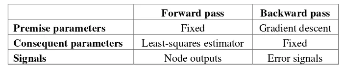
[image:30.595.135.485.174.244.2]

ANFIS have forward and backward passes of the hybrid learning algorithm. Table 2-8 summarizes the activities in each pass.

Table 2-8 ANFIS Learning (Jang, 1993)

Forward pass Backward pass

Premise parameters Fixed Gradient descent

Consequent parameters Least-squares estimator Fixed

Signals Node outputs Error signals

a) Forward Pass Learning

In the forward pass of the hybrid learning algorithm node outputs go forward until layer 4 and the consequent parameters are identified by the least-squares method. When the values of the premise parameters are fixed the overall output can be expressed as a linear combination of the consequent parameters.

2 1 2 2 2 2 1 1 1 1 1 1 2 1 1 1 ) ( ) ( ) ( ) ( ) ( )

(w x p w y q w r w x p w y q w r

f f w f w f        

Where, {p1, q1, r1, p2, q2, r2} are consequent parameters in layer 4. For given fix values of premise parameters, using K training data, it can transform the above equation into B=AX, where X contains the elements of consequent parameters. This is solved by: (ATA)-1AT B=X* where (ATA)-1AT is the pseudo-inverse of A (if ATA is nonsingular). The LSE minimizes the error ||AX-B||2 by approximating X with X*

b) Backward Pass Learning

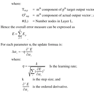
In the backward pass, the error signals propagate backward and the premise parameters are updated by gradient descent. Assuming the given training data set has P entries, we can define the error measure for pth (1 < p < P) entry of training data entry as the sum of squared errors:

2 , ) ( # 1 ,

)

(

_mL_p L

m

p m

p

T

O

E







13

where:

Tm,p = mth component of pth target output vector;

OLmp = mth component of actual output vector ; and

#(L) = Number nodes in Layer L. Hence the overall error measure can be expressed as



  P p p E E 1 _.

For each parameter αi the update formua is:

i i E          where:



_  i i E k 2 ) ( 

 Is the learning rate;

k is the step size; and

i E 

 

is the ordered derivative.

2.3.4 Related Research of ANFIS Prediction

[image:31.595.111.429.86.406.2]

There are some studies on classification or prediction using ANFIS algorithms (Table 2-9).

Table 2-9 Related Research of ANFIS

No Object Data Performance References

1 Oil Spill MODIS-Terra, MODIS

Aqua,Envisat-ASAR

under the ROC curve of 80%

Corucci et al., 2010

2 Crop Yield

Prediction

Statistical winter wheat data for 1999-2004

Overall Accuracy: 74%

Stathakis et al., 2006

3 Burnt area

by wildfires

MODIS-Terra, NOAA, Meteosat8

Prod Accuracy : 76% User Accuracy : 86%

Calado et al., 2006

[image:32.595.130.497.101.380.2]

14

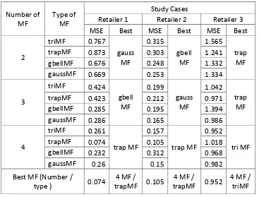
Table 2-10 Membership Function Comparison (Efendigil et al., 2009).

Number of MF

Type of MF

Study Cases

Retailer 1 Retailer 2 Retailer 3

MSE Best MSE Best MSE Best

2 triMF 0.767 gauss MF 0.315 gbell MF 1.565 trap MF

trapMF 0.873 0.303 1.241

gbellMF 0.676 0.248 1.332

gaussMF 0.669 0.253 1.334

3 triMF _0.424 gbell MF 0.199 gauss MF 1.042 trap MF

trapMF 0.423 0.212 0.971

gbellMF 0.285 0.195 1.394

gaussMF 0.286 0.165 0.986

4 triMF 0.261 trap MF 0.157 trap MF 0.952 tri MF

trapMF 0.074 0.105 1.018

gbellMF 0.232 0.312 0.968

gaussMF 0.26 0.15 0.982

Best MF (Number /

type ) 0.074

4 MF /

trapMF 0.105

4 MF /

trapMF 0.952

4 MF / triMF

2.3 Classification Accuracy

Error matrix is a square array of numbers set out in rows and columns that expresses the number of sample units assigned to a particular category in one classification relative to the number of sample units assigned to a particular category in another classification. Mathematical example of an error matrix is described in table 2-11.

Table 2-11 Error Matrixes (Congalton and Green 1999).

j = Columns (References) Row Total

1 2 k

n

i+

i=Rows (Classification)

1

n

11

n

12

n

1k

n

1+

2

n

21

n

22

n

2k

n

2+

k

n

k1

n

k2

n

kk

n

k+

Column Total

n

+j

n

+1

n

+2

n

+k

n

[image:32.595.150.471.561.682.2]

15 n n Accuracy Overall k i ii



  1 _ j jj n n j Accuracy s oducer   ) ( _ ' Pr   i ii n n i Accuracy s

User' _ ( )







          _k i i i k i k i i i ii n n n n n n n t Coefficien Kappa 1 2 1 1 _ where:



 k i ii

n

1

: The sum of major diagonal (the correctly classified sample unit);

n

: the total number of sample units; jj

n

: the total number of correct sample unit in “class x”; j

n

_

: total number of “class x” as indicated by the reference data; ii

n

: the total number of correct pixels in the “class x”; and



i

17

III.

METHODOLOGY

3.1 Time and Location

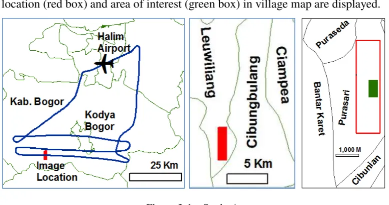
[image:35.595.112.502.263.469.2]

The study was conducted from November 2011 to July 2012 . The study case was in Purasari Villages – District of Leuwiliang - Bogor Regency. The location of study area can be seen in Figure 3. From this figure flight path of airborne line scanner flight in regency map, image location in district map, image location (red box) and area of interest (green box) in village map are displayed.

Figure 3-1 Study Area

3.2 Data Collection and Field Survey

3.2.1 Remote Sensing Data

The data used in this study were data from airborne line scanner taken on 3 November 2010. The data resulted into three images from Green, Red, and NIR channels. Data obtained from an altitude of approximately 2500 meters above mean sea level, with an average airborne speed of 120 knots, and ground resolution produced around 0.5 meter.

3.2.2 Field Survey Data

18

[image:36.595.127.496.271.458.2]

survey (6 days). This field observation was intended to label the names of classes. Tools used for the survey are GPS, manual compass, and an 8 megapixel camera. GPS type used was GPS-60 with accuracy + 15 meters. Thirty two points of GPS is taken together with fourth photos in each direction (North, South, West, and East). With GPS positioning error of 15 meters, a loop buffer with a radius of 15 meters was made. By utilizing photos with four directions the position was corrected using visual interpretation. Where taking pictures has always been on the field boundary and never was in the center of fields. Example of field survey data is described in Figure 3-2.

Figure 3-2 Example of Field Survey

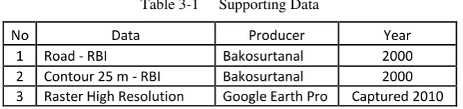
3.2.3 Supporting Data

For geometric correction, airborne line scanner data need supporting data. The resulting images on the flight test had a high resolution and are in agricultural areas, this is not possible to perform direct geo-referencing with road map - RBI or use the GPS data that has an error rate of more than one pixel. The geometry corrections must be conducted with raster that have been corrected with RBI map. Supporting data, which used in this research are shown in Table 3-1.

Table 3-1 Supporting Data

No Data Producer Year

1 Road - RBI Bakosurtanal 2000

2 Contour 25 m - RBI Bakosurtanal 2000

[image:36.595.146.480.662.741.2]

19

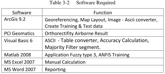
3.3 Software Required

[image:37.595.138.486.183.340.2]

This research needs some application software to process and training data. The application software’s for the overall processes in this study are described in Table 3-2.

Table 3-2 Software Required

Software Function

ArcGis 9.2 Georeferencing, Map Layout, Image - Ascii converter, Create Training & Test data

PCI Geomatics Orthorectifity Airborne Result

Visual Basic 6 ASCII - Table converter, Accuracy Calculation, Majority Filter segment.

Matlab 2008 Application Fuzzy type 3, ANFIS Training

MS Excel 2007 Manual Calculation

MS Word 2007 Reporting

3.4 Research Step

This research was done in some steps. They are image pre-processing, classification using ANFIS method, comparisons, and post-processing. The general methodology describes in figure 3-3.

[image:37.595.125.490.412.707.2]

20

3.4.1 Image Pre-Processing

Image pre-processing was done before image classification. There are two standard pre-processing, radiometric correction and geometric correction. Radiometric error due to sun angle and topography will be reduced by using image rationing. Atmospheric correction has not been used in this study, but it is expected will have no error contribution due to the low flying height.

For airborne line scanner, geometric correction was used for co-registration and geo-referencing. Co-co-registration was done for geometric correction of the green and red channels with reference to the NIR channel. NIR channel was chosen because the channel is the first time to take the pictures and the position closest to the center of gravity of the airborne. Because it is closest to the center of gravity, it has the smallest geometric error due to variations in airborne attitude. This camera is designed for satellite, and does not have stabilization mechanism. Result of this co-registration process was a composite image.

This composite image was geometric corrected using a map reference that has spatial data and DEM from contour RBI interpolation, with Ortho-rectification methods. All data used in this study were registered to RBI map. 3.4.2 Classification Using ANFIS Method

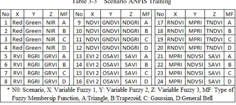
This study classified agricultural land covers using ANFIS method. From agriculture land, data can generate to original band (greed, red, & NIR) and image rationing band as described in Table 2-1. Training and validation data were made based on survey data. Refer to this survey; the classification was done in to 6 classes. These classes were fallow/non vegetation, new rice Planting, vegetative rice, reproductive rice, ripening rice, and trees.

21

Table 3-3 Scenario ANFIS Training

3.4.3 Comparison

Validation step was conducted to test the relationship between prediction and target output. The Error (confusion) matrix was used in this study to find the overall accuracy, producer’s accuracy, user’s accuracy, and kappa statistic for classification result. The sample data that were used for training process were not used in this accuracy assessment. Comparison between the scenarios results was determined by the kappa value, calculated from the error (confusion) matrix. The best scenario has been a scenario with the highest kappa value. The best scenario would eventually be used for classification or rice plant growth stage mapping. 3.4.4 Image Post-Processing

On the result of automatic classification, often found results that are not possible especially for high resolution images. Like object with a small area in the other object and object with strange pattern. For plant growth stage mapping, every segment of paddy field must be have one result. At post processing, the following procedures were applied:

1. Creating line boundary; 2. Converting line to polygon;

3. Calculating number of pixel each class in one polygon; and

[image:39.595.116.513.102.279.2]

23

IV.

RESULTS AND DISCUSSIONS

4.1 Image Pre-Processing

The main advantage of line scanner sensors is the ability to generate high resolution images without merging or stitching of images patches like in matrix imaging (Reulke et al., 2004). Line scanner camera has other advantages and disadvantages compared to other scanner types. These can be seen in Table 2-4. The main difference between matrix scanner and line scanner is on the time used for recording each row in images frame.

On matrix scanner, each line in the images is recorded at the same time. In line scanner, each line in the images is recorded at the different time. One thing that causes geometric error in the images is the camera stability. In matrix scanner, geometric errors pattern will occur in each images frame. In line scanner, geometric errors pattern will occur in each line of images frame. This fact cause the line scanner needs more ground control point (GCP) than matrix scanner for off nadir position.

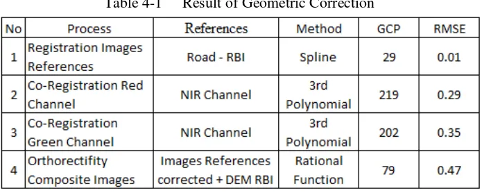
[image:41.595.139.488.539.678.2]

With less stable airborne attitudes and varying altitude of objects on earth, more than 200 control points for co-registration process were used. Number of control points used to obtain the least geometric error and good visualization. Detailed results of geometric correction are described in Table 4-1.

Table 4-1 Result of Geometric Correction

24

high quality geo-referenced image (Santhosh et al., 2011). Geometric correction produces corrected images with dimensions 917 x 2334 pixel and ground spatial distance 0.47 meter. A corrected image is shown in Appendix 1.

4.2 Field Survey

Congalton and Green (1999) stated that actual ground visitation may be the only reliable method of data collection. A subset of data should be collected on the ground and compared with the image data to verify the reliability of the image reference data. In this study the reference data were taken by visual interpretations that were then compared with field survey data.

25

Figure 4-1 Fallow/Non Vegetation Class

In Figure 4-1, fallow/non vegetation class consists of various objects, such as fallow with water cover, fields’ boundary, rocks, rivers, fish ponds, and another various objects with small area like grass in the river. Color of non vegetation in image maps can be distinguished easily with vegetation objects. Object without vegetation will be colored green and object with vegetation will be colored red.

[image:43.595.110.512.340.448.2]

New rice planting class is illustrated in Figure 4-2. Characteristics of new rice planting is has rare vegetation cover. With a resolution of around half meter, image color in the map is a combination of vegetative rice and fallow. The new rice planting class is early stages of paddy vegetative phase especially seeding until tillering stages (IRRI, 2012), due to the special characteristics of this object, it is classified separately.

Figure 4-2 New Rice Planting Class

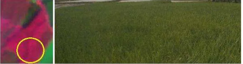
[image:43.595.116.514.559.664.2]

Vegetative rice class is illustrated in Figure 4-3. A characteristic of vegetative rice is to have dense vegetation. Color on visual observation is green uniforms and a color in an image map is a red uniform.

Figure 4-3 Vegetative Rice Class

26

[image:44.595.113.514.105.207.2]

of the survey is that the rice was still a flower.

Figure 4-4 Reproductive Rice Class

[image:44.595.114.512.333.482.2]

Ripening rice class is illustrated in Figure 4-5. Color on visual observation in this stage is dominantly yellow. Some land covers change during delay capture images and field survey (6 days) especially in this class. Some ripening rice changed to post harvest. This information obtained by interviewing farmers on the site.

Figure 4-5 Ripening Rice Class

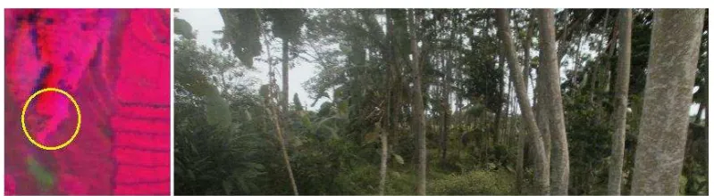
Trees class is illustrated in Figure 4-6. The study areas there are several kinds of trees. Trees class can be detected by looking at the color, images pattern, and survey data.

[image:44.595.113.513.587.697.2]

27

4.2.1 Compilation of Data Set

Compilation of data set consists of training data and validating data. The accuracy assessment reference data must be kept absolutely independent (i.e., separate) from any training/labeling data (Congalton and Green, 1999). Each training and validating data consists of 3 input from original images (NIR, red, green), 13 inputs from image rationing as shown in Table 2-1, and target data for training or references data for validating. The selected training areas should be homogeneous as much as possible.

[image:45.595.117.501.374.551.2]

The examples of training and validating area are described in Figure 4-7. The images also show training targets and references validating each class. Those classes are derived from field observations and taking into account the spatial resolution of remote sensing data. The area of training data sets are represented by each class type selected based on the ground reference points collected from the field supported by the local knowledge of the area.

Figure 4-7 Examples of Training and Validating Area.

[image:46.595.137.487.101.227.2]

28

Table 4-2 Number of Validating and Training Samples

4.3 Accuracy Assessment

4.3.1 Accuracy Assessment for Each Scenario

In this study, the same parameters have been used for each scenario. The parameters were three input and three membership functions (low, medium, and high), with epoch number = 1000, step size= 0.01, step size decrement Rate = 0.9, and step size increment rate = 1.1. Results of accuracy assessment for each scenario are described in Table 4-3.

Mather (2004) suggests that a value of kappa of 0.75 or greater shows a ‘very good to excellent’ classifier performance, while a value of less than 0.4 is ‘poor’. Congalton and Green, (1999) characterized the possible ranges for KHAT (kappa) into three groups: a value greater than 0.80 represents strong agreement; a value between 0.4 and 0.8 represents moderate agreement; and a value below 0.40 represents poor agreement.

[image:47.595.151.476.100.477.2]

29

Table 4-3 Scenario Comparison

30

One cause of low accuracy was due to the input statistics that were almost the same between classes. Input statistics of each class consisting of the average, minimum, maximum and standard deviation are shown in Appendix 3. From the data in Appendix 3 can be improved to normal distribution curve to see the possibility of different classes with the same value.

The normal distribution is a commonly occurring shape for population distributions. On normal distribution curve, the X axis represents different values for input, and the Y axis represents the density or the frequency or probability of occurrence of input. The total area under the curve is equal to 1. Normal distribution curve is shown in Appendix 4.

Normal distribution curve with red channel input overlapping occurs between ripening and new planting class. On green channel overlapping occurs between fallow with new planting class and ripening with trees class. On NIR channel overlapping occurs between ripening, trees, and vegetative class. These caused low accuracy in scenario 1 to 4.

4.3.2 Accuracy Assessment for Each Class

This section discusses the individual plant growth stages classes derived only from best scenario. The best scenario occurred from image rationing input. Accuracy assessment of each class is described in error matrix of training and error matrix of validating. Error on training matrix will create less precise Fuzzy Interference System (FIS) parameters to predict the targets from the input system. Error in the validation matrix demonstrates the ability of FIS to output predict which correspond to the actual class. Error matrix of training is described in Table 4-4 and Error matrix of validating is described in Table 4-5.

[image:49.595.115.511.90.258.2]

31

[image:49.595.115.512.91.449.2]

Table 4-4 Error Matrix of Training

Table 4-5 Error Matrix of Validating

In all normal distribution curves in Appendix 4, overlapping occurs between vegetative rice and reproductive rice class except in GNDVI. But in GNDVI overlapping occurs between reproductive with ripening class and vegetative with new planting class. On MPRI input, big overlapping only occurs between vegetative rice and reproductive rice class. These caused on reproductive rice and vegetative rice to have lower accuracy than ripening rice and new rice planting class. All inputs having similar the weakness, which clearly distinguishes between vegetative rice and reproductive rice. On NDVSI, big overlapping occurs between vegetative rice, reproductive rice, and trees class.

32

[image:50.595.147.481.168.274.2]

using MODIS Data (Domiri et al., 2005). The second study, modeled NDVI at the age of rice plants using ASTER Data (Nugroho et al., 2008). Results from both studies are depicted in Figure 4-8.

Figure 4-8 Vegetation Index of Rice from MODIS and ASTER

From Figure 4-8, vegetation index were possibly same value between before and after the 56 day. In the tropics, the reproductive phase is about 35 days and the ripening phase is about 30 days. The differences in growth duration are determined by changes in the length of the vegetative phase. For example, IR64 which matures in 110 days has a 45-day vegetative phase, whereas IR8 which matures in 130 days has a 65-day vegetative phase (IRRI, 2012). This was probably the cause of overlapping between vegetative, reproductive, and trees on the vegetation index such as NDVSI and SAVI.

33

4.3 Best Scenario of ANFIS Training

[image:51.595.113.512.108.312.2]

ANFIS uses a hybrid learning algorithm to identify parameters of fuzzy inference systems type 3. During the learning process, every epoch has RMS error and updates the step size. Error and step size curve are described in Figure 4-9.

Figure 4-9 Error and Step Size Curve

After the ANFIS learning process, premise and consequent parameters will be generated. Premise parameter is a parameter of membership degree which depend type of membership function. The initial value of membership function is calculated based on the statistics of the input training data. Final membership function is calculated based on ANFIS algorithm from input and target of training data. Initial and final membership function is described in Figure 4-10 and parameter of final membership function is described in Table 4-6.

[image:51.595.115.511.503.720.2]

[image:52.595.113.513.318.688.2]

34

Table 4-6 Parameter of Membership Function

In FIS type 3, the consequent is a crisp function of the antecedent variables. Fuzzy IF-THEN rule is a concept used for describing of logical dependence between variables of premise and consequent part. Rule and consequent parameters from best scenario is described in Table 4-7.

Table 4-7 Rule and Consequent Parameter

35

[image:53.595.139.487.177.232.2]

output value is exactly same as the target value of the class, except for the ANFIS training - RMS error is zero. To convert the float number to integer, range value is required. Target and range value of the class is described in the Table 4-8.

Table 4-8 Target and Range Value

After this process, the best scenario of ANFIS training for plant growth stage mapping was obtained. The best scenario of ANFIS training for plant growth stage mapping is shown in Appendix 6. The sample calculation of best scenario is shown in Appendix 7.

4.4 Rice Plant Growth Stage Mapping

Before calculating the area of rice plant growth stage, error correction should be done that cannot be avoided in automatic classification. Often, fully automated algorithms produce incomplete results so that manual post processing is inevitable (Kim et al., 2005). This section discusses the methods of classification results improved by giving a value to each segment based on the majority class. Object instance is vegetation rice in study area. The object is depicted in Figure 4-11.

[image:53.595.160.466.499.728.2]

36

[image:54.595.115.510.166.492.2]

Photo survey in Figure 4-11 in images is described in Figures 4-12. From the image, the boundary of each field is clearly visible, so that manual segmentation can be done. Each segment has an identification number (ID).

Figure 4-12 Post Processing

From the Figure 4-12, the results of classification still have errors such as ripening and reproductive rice. After class majority segment is used, each segment has one result. Calculation of majority class of each segment is described in Table 4-9.

[image:55.595.116.512.93.360.2]

37

Table 4-9 Statistic of Majority Class

The study area has been segmented as many as 1,172 pieces, with majority class average of 64.17%. Details of majority percentage of each segment are described in Figure 4-13. In Figure 4-13 has been sequenced from fallow class until trees class. Each class has been sorted from smallest to largest majority.

Figure 4-13 Majority Class Each Segment

[image:55.595.114.510.443.655.2]

38

39

V.

CONCLUSIONS AND RECOMMENDATIONS

5.1 Conclusions

The classification method have been developed using airborne line scanner data and ANFIS algorithm. This method has been applied to plant growth stage mapping. Data from airborne line scanner is quite good for distinguish of rice plant growth stage. ANFIS method is good enough to rice plant growth stage mapping from airborne line scanner.

Best accuracy results occurred in scenario with input images rationing (MPRI, NDVSI, and SAVI) with trapezoid fuzzy membership function, which gives kappa value 95.76%.

The predicted best class is paddy new planting and paddy ripening with producer’s accuracy of more than 97 % and user’s accuracy of more than 99% followed by paddy vegetative with producer’s accuracy of 93.98 % and user’s accuracy of 97.58 %. The class that predicted worse is paddy reproductive with producer’s accuracy of 78.61 % and user’s accuracy of 74.38 %.

5.2 Recommendations

Based on result there are several issues that can be further investigating to improve the results:

1. It may be worthy investigating different membership function in ANFIS. 2. It needs to compare with the result of applying the method to different

sensor with different spatial resolution, so that the accuracy obtained is more comprehensive.

3. Improvement may be obtained by combining the image and environmental data and compared with images rationing using the ANFIS method. 4. It is need for further researches to explore the ANFIS method for

41

REFERENCES

Abrams, J.M., 1983, Remote sensing for porphyry copper deposits in Southern Arizona. Economic Geology, 78, pp.591-604.

Salehi B.M. J., Valadan Zouj, 2004, Wavelet Spectral Analysis for Automatic Reduction of Hyperspectral Imagery , http://www.gisdevelopment.net/ technology/ip/mi04013.htm

Bertels, L., Deronde, B., Kempeneers, P., Provoost, S., Tortelboom, E., 2005; Potentials of airborne hyperspectral remote sensing for vegetation mapping of spatially heterogeneous dynamic dunes, a case study along the Belgian coastline; Interantional Conference on Nature Resporation Practices in European Coastal Habitats, Koksijde, Belgium, pp 153-163.

Calado, T.J., DaCamara, C.C. 2006, A synergetic use of remote-sensed data to assess the evolution of burnt area by wildfires in Portugal. The 2006 EUMETSAT Meteorological Satellite Conference, Helsinki, Finland, 12-16 June 2006, EUMETSAT P.48, ISBN 92-9110-076-5, 8pp

Congalton RG, Green K. 1999. Assesing the Accuracy of Remotely Sensed Data: Principle and Practices. New York:CRC Press, Inc.

Corucci Linda, Masini Andrea, 2010, Oil spill classification from multi-spectral satellite images using a neuro-fuzzy technique, IEEE GOLD Remote Sensing Conference, pp 1-3, Livorno, Italy.

Crane, R. B., 1971. Processing techniques to reduce atmospheric and sensor variability in multispectral scanner data. Proceed 7th. Int. Symp. Remote Sens. Environ., Ann Arbor, Vol.2, pp. 1345-1355

Dadhwal, V.K., 2004, Crop growth and productivity monitoring and simulation using remote sensing and GIS, Satellite RS and GIS Application in

Agriculture Meteorology, pp. 263-289.

Domiri D.D., Adhyani N.L.,Nugraheni S., 2005, Rice plant growth model using MODIS data for rice age prediction,Prosiding Pertemuan Ilmiah Tahunan MAPIN XIV, ISBN : 979-98982-1-8. pp 17-23.

42

Fletcher, R.S.; Everitt, J.H.; Elder, H.S. 2010, Evaluating Airborne Multispectral Digital Video to Differentiate Giant Salvinia from Other Features in Northeast Texas. Remote Sensing. 2010, 2, 2413-2423.

Gitelson, A.A., Y.J. Kaufman, and M.N. Merzlyak, 1996. Use of a green channel in remote sensing of global vegetation from EOS-MODIS, Remote Sensing Environment, 58:289-298.

Gong P., Biging G.S., Larrieu M.R., 2003. Estimation of forest leaf area index using vegetation indices derived from hyperion hyperspectral data, IEEE Trans. on Geoscience and Remote Sensing, Vol. 41, No. 6, June 2003. Hatfield J.L. Prueger J.H., 2010. Value of Using Different Vegetative Indices to

Quantify Agricultural Crop Characteristics at Different Growth Stages under Varying Management Practices. Remote Sensing. Vol.2, no. 2: 562-578.

Huete, A. R., 1988. A soil-adjusted vegetation index (SAVI), Remote Sensing of Environment, 25, 53-70.

Imdad A.R., Mohan B.K., 2010, Improving The Accuracy Of Object Based Supervised Image Classification Using Cloud Basis Functions Neural Network For High Resolution Satellite Images, International Journal Of Image Processing, ISSN 1985-2304 Volume 4.

IRRI [Internet]. 2012. International Rice Research Institute, Available:http://www.knowledgebank.irri.org/extension/three-growth-phases.html. Accessed July 2, 2012

Jang S.R., 1993, ANFIS: Adaptive-Network-based Fuzzy Inference Systems,

IEEE Transactions on Systems, Man, and Cybernetics, Vol. 23, No. 3, pp. 665-685.

Jiang Z., Huete A.R., Youngwook K., Kamel D., 2007. 2-band enhanced vegetation index without a blue band and its application to AVHRR data,

Proc. SPIE, Remote Sensing and ModelingTheory, Techniques, And Applications I, Vol. 6679, 667905.

Jordan, C.F., 1969. Derivation of leaf-area index from quality of light on the forest floor, Ecology, 50, pp. 663-666.

43

Kim T, Park S.R, Kim M.G, Jeong S, Kim K.O, 2005, Tracking road centerlines from high resolution remote sensing images by least squares correlation matching. Photogrammetric Engineering & Remote Sensing 70(12), 1417-1422.

Lillesand,T.M. and Kiefer,R.W, 1979, Remote Sensing and Image Interpretation, NewYork, Wiley. 2nd edition.

Mather P.M. 2004. Computer Processing of Remotely-Sensed Images . London: John Wiley & Sons Ltd

Monireh S.H. and Maryam Z., 2012, A review of medical image classification using Adaptive Neuro-Fuzzy Inference System (ANFIS), Journal of Medical Signal and Sensors Vol 2 No1

Nugroho D.A., Sukojo B.M., Wahyudi Y., 2008. Rice plants Identification with convert radians to the reflectance data in ASTER image, Prosiding Pertemuan Ilmiah Tahunan MAPIN XVII, ISBN: 978-979-25-8362-5. pp 117-130.

Panuju D.R., Trisasongko B.H, 2008, The Use Of Statistical Tree Methods On Rice Field Mapping, Jurnal ilmiah Geomatika Vol. 14 No.2, Bakosurtanal, Desember 2008

Patil V.C,Maru A, Shashidhara G.B. and U.K.Shanwad, 2002. Remote Sensing, Geographical Information System and Precision Farming in India: Opportunities and Challenges. http://www.jsai.or.jp/afita/afita-conf/2002/part6/p478.pdf pp 1-9

Reulke R., Wehr A., Griesbach D,2004, High Resolution Mapping Using CCD-line Camera and Laser Scanner with Integrated Position and Orientation System , International Society for Photogrammetric and Remote Sensing

volume XXXV, p. 506.

Rondeaux, G., M. Steven and F. Baret, 1996. Optimization of soil-adjusted vegetation indices, Remote Sensing of Environment, 55, pp.95-107.

Rouse, J. W., R. H. Haas, J. A. Schell, and D. W. Deering, 1973. Monitoring vegetation systems in the Great Plains with ERTS, Third ERTS Symposium, NASA SP-351 I, pp. 309-317.

Salem F., M. Kafatos, T. El-Ghazawi, R. Gomez, R. Yang, 2005. Hyperspectral image assessment of oil-contaminated wetland, International Journal Remote Sensing., Vol. 26, N 4, pp. 811-821

44

Sensed Imagery Using a Modified -NN Technique, IEEE Trans Geosci Remote Sensing 46(7):2112-2125.

Santhosh B. and Devi M.R., 2011, Geometric Correction in Recent High Resolution Satellite Imagery: A Case Study in Coimbatore, Tamil Nadu.

International Journal of Computer Applications 14(1):32-37, January 2011. Published by Foundation of Computer Science.

Stathakis D., SavinI.Yu., 2006. Neuro-fuzzy Modeling for Crop Yield Prediction, in the Proc. Of ISPRS Mid-term Symposium 2006 Remote Sensing: From Pixels to Processes Enschede The Netherlands.

Theta Aerospace, 2010, LAPAN LISA EM Glossary Training, LAPAN Internal Document.

Tjahjono B., A.H.A. Syafril, D.R. Panuju, A. Kasno, B.H. Trisasongko, F. Heidina, 2009, Rice field monitoring using ALOS AVNIR-2, Jurnal Ilmiah Geomatika, Vol 15 No.2, Bakosurtanal, Desember 2009

Tucker C.J., 1979. Red and photographic infrared linear combinations for monitoring vegetation, Remote Sensing of Environment, Vol. 8, pp. 127-150.

Wertz, James R.; Wiley J. Larson (1999). Space Mission Analysis and Design (3rd Ed. ed.). Kluwer Academic Publishers. ISBN 1-881883-10-8.

Yang Z, Willis P, Mueller R., 2008. Impact of band-ratio enhanced AWIFS image to crop classification accuracy, The Future of Land Imaging Going Operational, The 17th William T. Pecora Memorial Remote Sensing Symposium, Denver, Colorado.

45 Appendix 1 Corrected Image of Airborne Line Scanner

46

47

48

49

50

Appendix 5 3-D Scatter Graph of Training Data

51

52

Appendix 7 Sample of Calculation