Lithuania’s food demand during economic transition
Ferdaus Hossain
∗,1, Helen H. Jensen
2Rutgers University, 211 Cook Office Building, New Brunswick, NJ 08901-8520, USA
Received 13 June 1998; received in revised form 29 November 1999; accepted 29 December 1999
Abstract
The linear approximate version of the almost ideal demand system (LA-AIDS) model is estimated using data from the Lithuanian household budget survey (HBS) covering the period from July 1992 to December 1994. Price and real expenditure elasticities for 12 food groups were estimated based on the estimated coefficients of the model. Very little or nothing is known about the demand parameters of Lithuania and other former socialist countries, so the results are of intrinsic interest. Estimated expenditure elasticities were positive and statistically significant for all food groups, while all own-price elasticities were negative and statistically significant, except for that of eggs which was insignificant. Results suggest that Lithuanian household consumption did respond to price and real income changes during their transition to a market-oriented economy. © 2000 Elsevier Science B.V. All rights reserved.
Keywords:Transition economies; Food demand; LA-AIDS; Fixed effects model
1. Introduction
Since gaining their independence from the for-mer Soviet Union, Lithuania and other forfor-mer Soviet Republics, and other eastern European countries are experiencing major economic reforms. These reforms include privatization of property, liberalization of prices, and withdrawal of government subsidies for inputs and outputs. The market-oriented reform mea-sures have resulted in rapid increases in prices, severe erosion of real income and purchasing power, and ma-jor reallocation of resources within these societies. Al-though the transition policies have had effects specific
∗Corresponding author. Tel.:+1-732-932-9155;
fax:+1-732-932-8887.
E-mail address:[email protected] (F. Hossain)
1Ferdaus Hossain is Assistant Professor of Agricultural
Eco-nomics at Rutgers University.
2Helen Jensen is Professor of Economics at Iowa State
Univer-sity.
to each country, the general experience has been that, for the vast majority of the population in these coun-tries, the reforms have brought severe hardship through higher prices, lower real income, and lower real wages.
Lithuania was one of the early adopters of market-oriented economic reforms and its experience makes evidence from this country useful for on going evaluation of reforms for both Lithuania and other emerging market economies. In addition, Lithuania is one of the transition economies for which relatively detailed household surveys are available that provide information on income sources, demographics and consumption patterns of households. To date, very little is known about the consumption patterns of Lithuanian households and how households have ad-justed to the economic reform measures. The house-hold data provide a unique opportunity to obtain estimates of demand parameters that are important for other economic analyses.
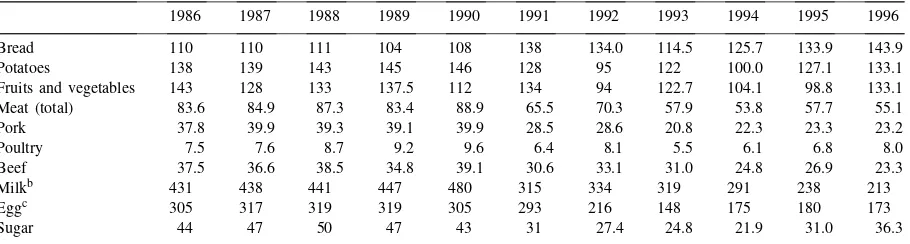
Table 1
Annual consumption of main food products, kg per capitaa
1986 1987 1988 1989 1990 1991 1992 1993 1994 1995 1996
Bread 110 110 111 104 108 138 134.0 114.5 125.7 133.9 143.9
Potatoes 138 139 143 145 146 128 95 122 100.0 127.1 133.1
Fruits and vegetables 143 128 133 137.5 112 134 94 122.7 104.1 98.8 133.1
Meat (total) 83.6 84.9 87.3 83.4 88.9 65.5 70.3 57.9 53.8 57.7 55.1
Pork 37.8 39.9 39.3 39.1 39.9 28.5 28.6 20.8 22.3 23.3 23.2
Poultry 7.5 7.6 8.7 9.2 9.6 6.4 8.1 5.5 6.1 6.8 8.0
Beef 37.5 36.6 38.5 34.8 39.1 30.6 33.1 31.0 24.8 26.9 23.3
Milkb 431 438 441 447 480 315 334 319 291 238 213
Eggc 305 317 319 319 305 293 216 148 175 180 173
Sugar 44 47 50 47 43 31 27.4 24.8 21.9 31.0 36.3
aSource: data for 1986–1991 period come from OECD (1996) and those for the 1992–1996 period from FAO data, FAOSTAT. The
data come from the Food Balance Sheet for Lithuania at http://apps.fao.org.
bFAO data for milk represent fluid milk, whereas OECD figures for milk represent fluid milk plus milk equivalent of other dairy
products. For consistency, milk consumption data for the 1992–1996 period were obtained from the Department of Statistics, Lithuanian Ministry of Agriculture through personal contact.
cConsumption of eggs is measured in number per capita.
Lithuania was among the most developed and in-dustrialized economies of the former Soviet Union, with per capita gross domestic product (GDP) in the 1990s about 50% higher than that of Russia (OECD, 1996). Following the adoption of price liberalization, however, the GDP fell significantly after 1990 before showing signs of growth in 1994. Prices increased sharply during 1991 and 1992. The official annual in-flation rate soared to 383% in 1991 and 1163% in 1992 before moderating to 45% in 1994 and 36% in 1995 (OECD, 1996). Real wages in the public sector fell dramatically through 1993 and since then have im-proved slightly (OECD, 1996). Initially, increases in wages and social benefit payments partly compensated for the price increases. But budgetary pressure made it increasingly difficult for the government to increase social benefit payments in line with price increases.
The average level of food consumption in Lithua-nia during the late 1980s was quite high, especially relative to per capita income. Consumption of milk and milk products was particularly high. The high per capita consumption reflected both abundance of sup-ply and a high consumer subsidy that resulted in low prices at retail levels. Following the liberalization of prices, however, as output of livestock products fell, prices rose sharply and consumption dropped dramat-ically. Between 1990 and 1996, per capita consump-tion of beef, pork and eggs fell by more than 40%, and milk consumption fell by about 36%, whereas
that of potatoes declined by about 13%, as shown in Table 1. On the other hand, per capita consumption of grain-based products increased. Per capita consump-tion data thus suggest that, as relative prices changed and real income fell, consumption of relatively expen-sive products declined. Specifically, grains, fruits, and vegetables were substituted for more expensive food items.
This paper reports the results of an analysis of consumption expenditures of Lithuanian households during the economic transition period of the 1990s. Using a panel structure of the household budget sur-vey (HBS) data and linear approximation version of the almost ideal demand system (LA-AIDS) model of Deaton and Muellbauer (1980), demand system parameters are estimated. The plan of the paper is as follows: Section 2 describes the data and panel con-struction; model specification and estimation methods are outlined in Section 3; and empirical results are presented in Section 4, followed by a concluding section.
2. Data
Soviet Family Budget Survey (Atkinson and Mick-lewright, 1992). The design included monthly surveys of households where households were included in the survey for 13 months. This allowed for a sam-ple rotation with 1 of every 13 households replaced each month. The stratified survey design included samples from urban (Vilnius and other urban areas) and rural areas and from different income levels. The income levels were set by ad hoc intervals in 1992 and 1993, and by deciles in 1994 (Cornelius, 1995). Although the HBS marked a significant improvement over the earlier survey, in practice, the implementa-tion suffered from certain weaknesses associated with the sample not being fully random as well as from non-response because not all households completed the full 13-month period of inclusion in the survey design. In total, about 1500 households were surveyed in each month. Despite the problems, the 1992–1994 HBS provides current and complete consumption and expenditure data for the period of interest. Review of the data with other, aggregated consumption data did indicate the data to be a good measure of con-sumption trends and representative of the national population.
2.1. Panel data construction
As mentioned earlier, all households did not com-plete the full 13-month period of inclusion in the sur-vey. The procedure for household replacement (re-placement of a household dropping out of the sur-vey by another household of similar type) was not tightly controlled or properly recorded during the sur-vey. Consequently, the survey design does not allow for uniquely identifying households from month to month for construction of a panel of data at the house-hold level. Alternatively, for this analysis, monthly household data for the period July 1992 through De-cember 1994 were used to create panel data for 40 representative household groups, defined by house-hold size, level of total (per capita) expenditures, and location (rural/urban).
The panel of the 40 representative household groups was constructed as follows. First, households were classified into five quintiles on the basis of per capita total household expenditures. Second, within each per capita expenditure quintile, households were classified into rural and urban households. This
two-level classification (quintiles and rural/urban) yielded 10 household groups (5×2). Third, each group of households was then further classified according to household size. This third-level classification took into account the distribution of household sizes in the whole sample and yielded a reasonably balanced distribution of observations in different cells in the three-level classification. Once the classes were se-lected, the means of different variables in each of the cells were used as representative values of the cor-responding variables in the data set. This procedure generated 40 observations for each of the 30 months of data, and for a total of 1200 observations.
2.2. Prices and expenditures
The survey instrument was used to collect detailed information on household expenditures for various food and non-food commodities and services, as well as demographic and income data. Information was collected on more than 65 food items for each month, during which time, households reported their weekly expenditures and corresponding quantities on each of the food items. The nominal expenditure was di-vided by quantity data to obtain a unit-value. The unit-values of different food items were used as prices. However, because observed variations in unit-values across households could be due to quality differences as well as actual differences in price distributions, the average (mean) unit-value of a commodity was used as the price that all households faced. Separate prices were computed for rural and urban house-holds to allow for price variation across the two re-gions (rural/urban). It was implicitly assumed that all households within the same region (rural/urban) and at any particular point in time faced the same set of prices.
sepa-rately for rural and urban households by using appro-priate unit-values. Non-purchased food represented about 30% of total food expenditure for rural holds and a slightly lower share for urban house-holds.
For estimation purposes, expenditures on various food commodities were aggregated into 12 categories: grains, fruits and vegetables, beef, pork, poultry, eggs, other meat products (including processed meat), fluid milk, butter and cheese, other dairy products, sugar and confectionery items, and other food (which in-cludes fats, fish, spices, non-alcoholic beverages, and other minor items). Expenditure shares on fat and fish were found to be small; consequently, a deci-sion was made to relegate them to the other food category.
3. Model and empirical specification
The conceptual framework and empirical specifi-cation of the demand system took advantage of the panel structure of the data to account for variation across households and over time. Ideally, in order to be able to make unconditional inferences about the population from which the sample of households was drawn, one should use a random effects model. However, estimation of the random effects model requires cross-sectional variation in all explanatory variables. In addition, a random effects model is ap-propriate if the individual effects are uncorrelated with other regressors in the model. In the data set used in this study, there is no cross-sectional variation in prices; only household expenditures vary across cross-sectional units. The fact that only one regres-sor (i.e., expenditure) has cross-sectional variation suggests that several key household-specific variables have been omitted, and their effects get combined into the household-specific intercept terms, theindividual effects. This in turn makes it more likely that these individual effects are correlated with the one regres-sor that does vary across households. In addition, as discussed earlier, the survey design used to collect household data resulted in the sample being not fully random.
On account of these factors, a decision was made to estimate the fixed effects model (otherwise known as the least squares dummy variables (LSDV)
model).3 In this framework, the effects of cross-sectional variation (effects of variables that vary across households but remain fixed over time) and time-specific effects (effects of variables that are the same across households but change over time) were captured by allowing the intercept terms of the demand equations to vary across cross-section and across time.
The LA-AIDS of Deaton and Muellbauer (1980), that uses Stone’s (expenditure) share-weighted price index instead of the non-linear general price index of the full AIDS model, is used to estimate the de-mand system. The LA-AIDS model is augmented to incorporate the effects of cross-sectional variation and time-specific effects. The cross-sectional (hence-forth household effect) and the time-specific effects (henceforth time effect) are assumed to be fixed in the LSDV version of the LA-AIDS model. Apart from its aggregation properties that allow interpretation of the demand parameters estimated from household data to be equivalent to those estimated from aggregate data, the LA-AIDS model is popular in empirical analysis because of the model’s linearity in terms of its parameters.
The AIDS model is derived from an expenditure function and can be expressed as
wi =αi∗+ K X
j=1
γij∗lnpj+βi∗ln x
P
+ηi, (1)
wherewi is the expenditure share of theith good,pj is the price of the jth good, xis the total (nominal) expenditure on food,ηiis the error term, and lnPis the general price index which, in the case of the LA-AIDS model, is approximated by the Stone’s price index as
lnP =
K X
j=1
wjlnpj. (2)
Denotingreal expenditure, (x/P), by y, and augment-ing Eq. (1) to incorporate the household and time ef-fects, the LSDV version of the LA-AIDS model can be expressed as
3 The use of fixed effects model rather than the random effects
wiht=αi+µih+λit+ K X
j=1
γijlnpj t+βilnyht+uiht,
h=1,2, . . . , H, t =1,2, . . . , T . (3)
where wiht is the expenditure share of the ith food group for household h specific to time period t, αi is the average intercept term (for the ith good), µih represents the difference betweenαi and the intercept term corresponding to theith good and thehth house-hold, and λit is the difference between αi and the intercept term for theith good and thetth time period. At any given time period, the parameterµihcaptures the influence (on the demand for the ith good) of the variables that vary across households but remain constant over time. The parameter λit reflects the influence (on the demand for the ith good) of those factors that are common to all households and change over time. The household effects (µih) and time
ef-fects (λit) are assumed to be fixed. There areH num-ber of cross-sectional units (households) andT time periods. It assumed that the vector of disturbances corresponding to theith good and thehth household, uih, has the property thatE[uih]=0, E[uihu′ih]=σi2I (σi2 is the variance corresponding to ith equation),
andE[uihu′ij]=0 forh6=j. To satisfy the properties of homogeneity, adding-up, and Slutsky symmetry, the parameters of Eq. (1) are constrained byP
iαi =1, P
iβi =0,Piγij =Piγj i =0,andγij =γij. Fur-ther, to avoid the dummy variable trap in the LSDV model, the above model is estimated with restrictions P
hµih=0 andPtλit =0.4
The demand system is estimated under the implicit assumption that households treat market prices as pre-determined. Although the study covers a period when there were supply disruptions and significant price in-creases, we assume that individual households acted as if their individual purchase decisions did not have an effect on market prices. Under this assumption, con-sumption demand was modeled with prices taken as predetermined.
The LA-AIDS formulation is not derived from any well-defined preferences system, and is only an ap-proximation to the non-linear AIDS model. Moschini (1995) demonstrates that the Stone’s price index is not
4See Judge et al. (1985) (chapter 13) for discussion of the
estimation procedure.
independent of the choice of any arbitrary unit of mea-surement for prices. Consequently, the estimated pa-rameters from the LA-AIDS model based on Stone’s price index may contain undesirable properties. To avoid such potential problems, we follow Moschini’s (1995) suggestion to define the price indices for each commodity group in units of the mean of the price series (i.e., pj∗ = (pj/µpj), where pj is the price
index of commodity group j, and µpj is the mean
ofpj).
3.1. Model estimation
The demand system model (Eq. (3)) is estimated with the data set described in Section 2. In keeping with the restrictions of the AIDS model, one equation is deleted in the estimation process. The model is esti-mated with dummy variable restrictions along with the homogeneity and Slutsky symmetry restrictions (i.e., P
jγij = 0, andγij=gj i) as a maintained
hypothe-ses. Since the observations of the panel data used to estimate the above system are group averages, the use of these averages directly in the estimation would lead to heteroscedasticity unless all group sizes are equal. In order to correct for this problem, each of the vari-ables in the data set is transformed as
z∗g =√ngzg (4)
where the subscriptgrefers to the groupg, andngis the number of households in groupg. The transformed variables are then used to estimate the coefficients of the demand model.
4. Empirical results
statistical tests did not show evidence of heteroscedas-ticity and serial correlation.5
The estimated coefficients of the demand system along with thet-ratios are reported in Table 2. Other coefficients of the system, including those of the deleted equation, can be recovered from the restric-tions imposed in the estimation process. As shown in Table 2, most of the estimated coefficients are statisti-cally significant at the 5% level. Also, it can be noted from the last column of Table 2 that the coefficients of real expenditure are statistically significant for all commodity groups. Similarly, all of the own-price effects are statistically significant, as shown along the diagonal of Table 2. But economic theory does not imply any particular sign for any of the coefficients as these coefficients are associated with the logarithm of prices rather than levels of prices.
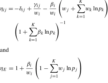
The elasticities of demand (price and expenditure elasticities) were estimated by the methodology sug-gested by Green and Alston (1990, 1991). The Mar-shallian (uncompensated) elasticities for the LA/AIDS model are derived as6
ηij= −δij +
The estimated uncompensated (Marshallian) elas-ticities along with their t-ratios are presented in Table 3. Thet-ratios were estimated using bootstrap-ping methods at mean levels of prices and
expendi-5Bartlett’s test (see Judge et al., 1985: p. 447) on the residuals
from each equation did not suggest the presence of heteroscedas-ticity. Also, a test of serial correlation did not indicate any evi-dence of the problem.
6There is some disagreement in the literature regarding the
appropriate formula for estimating elasticities in the LA-AIDS model. This is due to the fact that the LA-AIDS model is only a linear approximation of the full AIDS model (see Hahn (1994) and Buse (1994) on this issue).
tures. Based on the model specification, these elastic-ities should be interpreted as conditional elasticelastic-ities where it is assumed that the relative price changes within the food groups do not affect the real expen-diture on food. Also, it is implicitly assumed that short-run dynamics in the adjustment of food expen-diture patterns have been fully incorporated within the time period.
5. Discussion
The estimated price and expenditure elasticities seem to be reasonable: all own-price elasticities are negative and statistically significant except for that of eggs. Most of the cross-price elasticities are statisti-cally significant and many of them are positive. All expenditure elasticities are positive and statistically significant. It may be noted that expenditure elastici-ties for grains, eggs, fluid milk, butter and cheese, and other dairy products are less than unity, indicating that consumers treat these commodities as essentials. On the other hand, expenditure elasticities for beef, pork, poultry, sugar and confectionery items, and other food items are higher than unity, whereas those for fruits and vegetables and other meat (including processed meat) are slightly above unity. This suggests that, as real income of the consumers fell, major consump-tion reducconsump-tions came in the meat (except processed meat products, identified as other meat), sugar and confectionery items, and other food items. Expen-diture reductions on fruits and vegetables and other meat were almost proportional to the income decline. On the other hand, expenditure on grains, eggs and various dairy products fell less than proportionately as real income was eroded by inflation. This is not surprising given the economic hardship experienced by the people of Lithuania during the period under consideration. The estimated expenditure elasticities are relatively high compared to those found in most developed countries, and they are comparable to those found for less developed societies. In that sense, the relatively high expenditure elasticities are reflective of the economic condition of Lithuanian households during the transition period.
the own-price elasticities are less than unity as is expected for food commodities. These elasticities are expected to be low for essential commodities and relatively high for commodities that are notessential items. This is reflected by the low estimated own-price elasticities for grains (−0.44), other dairy (−0.51), and fluid milk (−0.59), and relatively high elastici-ties for pork (−1.92), other food (−1.35), butter and cheese (−1.49), and other meat (−1.12). Estimated cross-price elasticities suggest that consumption of grains did not respond to changes in dairy product prices; demand for various meat categories was in-sensitive to changes in the price of poultry (which account for about 10% of total meat consumption); and consumption of fruits and vegetables was unaf-fected by changes in the prices of meat and dairy products. Other cross-price elasticities seem to be reasonable both in terms of their magnitudes as well as their signs.
Although the parameter estimates and estimated price and expenditure elasticities seem reasonable based on other studies on consumption, it is difficult to compare these estimates with others because few studies on the consumption patterns of the formerly socialist societies exist. Also, the period under con-sideration is one during which the society as a whole underwent significant economic and political change with supply disruptions and price increases. Also, it should be noted that the parameters and elasticities are estimated under the assumption that the food consumption depends on the amount of (real) income devoted to food commodities (i.e., the utility function is at least weakly separable). Therefore, the estimates are essentially conditional estimates. Other estimates by the authors found the expenditure elasticity for food estimated in a total demand system to be 0.98.
5.1. Other tests
The empirical results presented previously are based on the model specified in Eq. (3) which assumes that cross-section household units and time variation have important effects on household food expenditure pat-terns. This assumption can be verified by testing with a standardF-test the null hypothesis that all µihand
λit coefficients are simultaneously equal to 0. The test yielded an estimated value of the test statistic equal to 23.85, which exceeds the 95% critical value of the
F-distribution (with appropriate degrees of freedom). Hence, the null hypothesis of no cross-section and time effects is rejected at a conventional significance level. The estimated demand system incorporates the zero-degree homogeneity and symmetry restrictions as implied by economic theory. The a priori imposi-tion of the zero-degree homogeneity restricimposi-tion pre-supposes that the consumers do not suffer frommoney illusion. The fact that the data for this study cover a period during which Lithuania experienced large ab-solute and relative price changes makes formal testing of the assumption all the more interesting. Accord-ingly, we tested for the validity of the assumption of the (zero-degree) homogeneity of the demand system. The formal test uses the likelihood ratio test for the system as a whole and theF-test for individual equa-tions. The likelihood ratio test yielded an estimated test statistic of 395.6, which exceeds the 95% critical value of the Chi-square distribution (with appropriate degree of freedom), implying that the system as a whole did not satisfy the zero-degree homogeneity restriction. The results from theF-test for individual equations revealed that only three commodity groups (namely poultry, sugar and confectionery items, and other food) satisfied the restriction at a 5% level, while the restriction could not be rejected at the 1% level for fruits and vegetables, beef, and other meat. Test results for all other groups contradicted the validity of the zero-degree homogeneity restriction and suggest the presence of money illusion for many of the food groups. Finally, the likelihood ratio test of homogene-ity and (Slutsky) symmetry restrictions yielded a test statistic of 769.2, which exceeded the 95% critical value of the Chi-square distribution (with appropri-ate degrees of freedom). This indicappropri-ates that the data reject the homogeneity and symmetry restriction as implied by economic theory.
6. Conclusion
as consumers substituted less expensive grain-based items, as well as fruits and vegetables.
Household consumption data reveal that, during the transition period examined here, households were responsive to changes in prices and household pur-chasing power. Estimated expenditure elasticities were positive and statistically significant for all food groups as is expected. The magnitudes of the mated elasticities, however, are higher than those esti-mated for developed countries. These magnitudes are consistent with those found in relatively low-income countries and reflect the economic hardship faced by Lithuanian households. The estimates suggest that expenditures on commodities such as beef, pork, and sugar and confectionery items fell rather significantly while those for grains, eggs, and miscellaneous dairy products fell less than proportionately. Price elastici-ties for the major food groups are also relatively high compared to those found in developed countries de-spite allowances for home production of food. This finding indicates that demand for food commodi-ties in Lithuania is quite price sensitive. Estimated cross-price elasticities suggest that, as relative prices changed, households adjusted their food consumption patterns through substitution among competing food items.
Acknowledgements
This research was conducted under a collaborative research agreement with the Lithuanian Department of Statistics and the Ministry of Social Welfare. We
acknowledge especially the advice and data provided by Zita Šniukstiené of the Department of Statistics. This is Journal Paper No. 17954 of the Iowa Agricul-ture and Home Economics Experiment Station, Ames, IA, Project No. 3513 and supported by Hatch Act and State of Iowa Funds.
References
Atkinson, A.B., Micklewright, J., 1992. Economic Transformation in Eastern Europe and the Distribution of Income. Cambridge University Press, Cambridge.
Buse, A., 1994. Evaluating the linearized almost ideal demand system. Am. J. Agric. Econ. 76, 781–793.
Cornelius, P.K., 1995. Cash benefits and poverty alleviation in an economy in transition: the case of Lithuania. Comp. Econ. Stud. 37, 49–69.
Deaton, A.S., Muellbauer, J., 1980. An almost ideal demand system. Am. Econ. Rev. 70, 312–326.
Green, R., Alston, J., 1990. Elasticities in AIDS models. Am. J. Agric. Econ. 72, 442–445.
Green, R., Alston, J., 1991. Elasticities in AIDS models: a clarification and extension. Am. J. Agric. Econ. 73, 874–875. Hahn, W.F., 1994. Elasticities in AIDS models: comment. Am. J.
Agric. Econ. 76, 973–977.
Judge, G.G., Griffiths, W.E., Hill, R.C., Lütkepohl, H., Lee, T., 1985. The Theory and Practice of Econometrics. Wiley, New York.
Moschini, G., 1995. Units of measurement and the stone price index in demand system estimation. Am. J. Agric. Econ. 77, 63–68.
Organization for Economic Co-operation and Development (OECD), 1996. Review of Agricultural Policies: Lithuania. Paris, France: OECD, Center for Co-operation with the Economies in Transition, Paris.