DEVELOPING TOOLS FOR COMPUTATION OF BASIN TOPOGRAPHIC
PARAMETERS IN GIS
T. Gökgöz*, Y. Yayla, M. B. Yaman, H. Güvenç, S. Kaya
Dept. of Geomatic Engineering, Yıldız Technical University, 34220 Esenler Istanbul, Turkey – [email protected], (yclyayla55, bahadir543, huseyinguvenc93, serhat.ky56)@gmail.com
Commission VI, WG VI/4
KEY WORDS: Shape Factor, Bifurcation Ratio, Drainage Frequency, Drainage Density, Harmonic Slope, Average Slope, Time of Concentration, Hypsometric Curve
ABSTRACT:
Although water use has been increasing day by day depending on fast population increase, urbanization and industrialization in the world, potential of usable water resources remains stable. On the other side, expansion of agricultural activities, industrialization, urbanization, global warming and climate change create a big pressure on current water resources. Therefore, management of water resources is one of the most significant problems of today that is required to be solved and ‘’Integrated Basin Management’’ has gained importance in the world in terms of decreasing environmental problems by more efficiently using current water resources. In order to achieve integrated basin management, it is needed to determine basin boundaries with sufficient accuracy and precision and encode them systematically. In various analyses to be done on the basis of basin, topographic parameters are also needed such as shape factor, bifurcation ratio, drainage frequency, drainage density, length of the main flow path, harmonic slope, average slope, time of concentration, hypsometric curve and maximum elevation difference. Nowadays, basin boundaries are obtained with digital elevation models in geographical information systems. However, tools developed for topographic parameters are not available. In this study, programs were written in Python programming language for afore-mentioned topographic parameters and each turned into a geographical information system tool. Therefore, a significant contribution has been made to the subject by completing the deficiency in the geographical information system devoted to the topographic parameters that are needed in almost every analyses concerning to the hydrology.
* Corresponding author
1. INTRODUCTION
The concept of a watershed is basic to all hydrologic designs. Since large watersheds are made up of many smaller watersheds, it is necessary to define the watershed in terms of a point; this point is usually the location at which the design is being made and is referred to as the watershed “outlet.” With respect to the outlet, the watershed consists of all land area that sheds water to the outlet during a rainstorm. Using the concept that “water runs downhill,” a watershed is defined by all points enclosed within an area from which rain falling at these points will contribute water to the outlet. Given this definition of a watershed and assuming that the delineation of a watershed is important to hydrologic design, it is necessary to show how the boundary of a watershed is delineated. Keeping in mind that the boundary of a watershed is defined by all points that will shed water to the outlet, it is only necessary to decide which points in a region will contribute water to the outlet; the most extreme of these points represents the watershed boundary (McCuen, 1998).
2. METHODS
The watershed shape factor is computed as the square of the length of the main flow path divided by the watershed area. It is understood that the bigger the shape factor is, the longer and narrower the watershed will be. Inputs of shape factor program are watershed and stream network. The bifurcation ratio is
computed based on the ordering that is done according to Horton’s method. The stream order is a measure of the degree of stream branching within a watershed. Each length of stream is indicated by its order (for example, first-order, second-order, etc.). A first-order stream is an unbranched tributary, and a obtained by arithmetically averaging all bifurcation ratio. The inputs of bifurcation program are watershed, flow direction and stream definition. The drainage frequency is defined as the total number of stream segments per unit area. The stream segments with same Horton’s order that have been transformed into vector data are intersected with the watershed layer. The drainage frequency is computed in the form of ratio of total stream segments with same Horton’s order obtained to watershed area. The inputs of drainage frequency program are watershed, flow direction and stream definition layers. The drainage density is the ratio of the total length of streams within a watershed to the total area of the watershed. It is understood that the total length of streams within that watershed per unit will be high in case drainage density is high. This means that the rain falling on the watershed from the troposphere will reach the watershed outlet in The International Archives of the Photogrammetry, Remote Sensing and Spatial Information Sciences, Volume XLII-2/W1, 2016
3rd International GeoAdvances Workshop, 16–17 October 2016, Istanbul, Turkey
This contribution has been peer-reviewed.
the shortest time. In case drainage density is high, flow risk will be less but percolation of water to the underground will be high. The higher the drainage density is, the longer the transfer rate of the water to the watershed outlet will be. The inputs of drainage density program are watershed and stream network. The distance measured along the main flow path from the watershed outlet to the end of the main flow path is the length of the main flow path. The inputs of length of main flow path program are watershed and stream network. Flood magnitudes reflect the momentum of the runoff. Slope is an important factor in the momentum. Both watershed and channel slope may be of interest. Watershed slope reflects the rate of change of elevation with respect to distance along the main flow path. Typically, the main flow path is delineated, and the watershed slope is computed as the difference in elevation between the end points of the main flow path divided into ten equal parts. By overlaying these parts with digital elevation model, elevations at the end points of each part are determined. The harmonic slope is computed by using the slope values obtained. As the harmonic slope is computed by dividing the main flow path into parts, it yields a more sensitive result compared to average slope in time concentration. The inputs of harmonic slope program are watershed, stream network and digital elevation model. The average slope is computed by using the parts within watershed boundary of digital elevation model. The slope map is produced from digital elevation model and average slope value is obtained as one of zonal statistics. The inputs of average slope program are watershed and digital elevation model. Time of concentration is a fundamental watershed parameter. It is used to compute the peak discharge for a watershed. The peak discharge is a function of the rainfall intensity, which is based on the time of concentration. Time of concentration is the longest time required for a particle to travel from the watershed divide to the watershed outlet. The equation used in our time of concentration computation require inputs for the length of main flow path, the harmonic slope, and a coefficient representing the type of ground cover. The inputs of time of concentration program are watershed, stream network and digital elevation model. The hypsometric curve is a description of the cumulative relationship between elevation and the area within elevation intervals. The curve is plotted with the elevation plotted as the ordinate and the area within the watershed above the elevation plotted as the abscissa. The hypsometric curve can also be represented in standardized form, with the cumulative fractions plotted rather than the actual values. The standardized form is useful for comparing the area-elevation characteristics of watersheds. Such comparison might be useful if a regional hypsometric curve were being developed from the analysis of hypsometric curves of watersheds in the region; after standardizing the hypsometric curves for each watershed, an ‘average’ curve could be constructed for the region. Where the necessary data are not available at other watersheds in the region, the regional hypsometric curve could be used to represent the area-elevation characteristics of the watershed (McCuen, 1998; Şen, 2002; Aslan, 2005; Akar, 2009). In this study, the digital elevation model is classified according to elevation interval determined. In the digital elevation model classified, number of cells in every class are determined. Number of cells in every class is multiplied with a cell area and thus area of every class is computed. These area values are counted up cumulatively. The elevation data are also classified in the same way. The hypsometric curve is created with the area and elevation values obtained. While assessing the curve formed, approximately 10% parts are deducted from start and end of the curve. The inputs of hypsometric curve program are
watershed, digital elevation model and elevation interval. Maximum elevation difference is the vertical distance between the outlet and the point with highest elevation of the watershed. It is computed in the form of the difference between minimum and maximum values of digital elevation model within the watershed boundary. The inputs of maximum elevation difference program are watershed and digital elevation model. All of the outputs of the programs that are computed as explained above are added to the watershed table as new attributes (Zandbergen, 2013).
3. RESULTS AND CONCLUSIONS
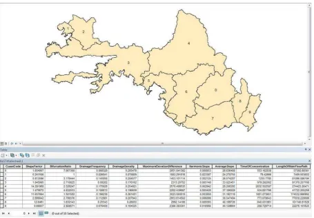
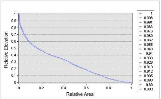
The implementation region is Western Mediterranean Basin that is located at middle latitude zone (between 36.13 and 37.67 degree latitudes), east-west elongated (between 27.23 and 30.59 degree longitudes) and that is a very big basin (approximately 20,554.82 km2) (Figure 1). In the implementation, digital elevation model with 10 meters geometrical resolution, drainage network and basin boundaries that were produced with the analyses on this digital elevation model were used. Western Mediterranean Basin is composed of ten sub-basins at first level. All afore-mentioned topographical parameters were computed for these sub-basins (Figure 2). The elevation and area ratio values that were computed with 10 meters intervals were normalized between 1 and 0 and hypsometric curve was formed for each sub-basin. The hypsometric curve that was formed for the sub-basin with the coast code 2 is given in Figure 3. When topographic parameters and hypsometric curves are examined, it is understood that the sub-basin with the coast code 2 is a very inclined, narrow and long basin. Also, it indicates a low flood risk that it has high drainage density.
ACKNOWLEDGEMENTS
The authors would like to thank the Scientific and Technological Research Council of Turkey (TUBITAK) for the financial support given under Project No: 115Y411.
REFERENCES
Akar, İ., 2009. How Geographical Information Systems and Remote Sensing are used to Determine Morphometrical Features of the Drainage Network of Kastro (Kasatura) Bay Hydrological Basin. International Journal of Remote Sensing. 30(7), pp. 1737–1748.
Aslan, Ş. T. A., 2005. Determination of Some Watershed Characteristics Using Geographical Information System Features. KSU Journal of Science and Engineering. 8(2), pp. 128-134.
McCuen, R. H., 1998. Hydrologic Analysis and Design. Prentice Hall, New Jersey, pp. 97-171.
Şen, Z., 2002. Basic Elements of Water Science. Su Vakfı, Istanbul, pp. 31-46.
Zandbergen, P. A., 2013. Python Scripting for ArcGIS, Esri Press, USA.
The International Archives of the Photogrammetry, Remote Sensing and Spatial Information Sciences, Volume XLII-2/W1, 2016 3rd International GeoAdvances Workshop, 16–17 October 2016, Istanbul, Turkey
This contribution has been peer-reviewed.
Figure 1. Western Mediterranean Basin
Figure 2. Sub-basins at first level of Western Mediterranean Basin and their topographic parameters
The International Archives of the Photogrammetry, Remote Sensing and Spatial Information Sciences, Volume XLII-2/W1, 2016 3rd International GeoAdvances Workshop, 16–17 October 2016, Istanbul, Turkey
This contribution has been peer-reviewed.
Figure 3. Hypsometric curve created for the sub-basin with the coast code 2 at first level of Western Mediterranean Basin The International Archives of the Photogrammetry, Remote Sensing and Spatial Information Sciences, Volume XLII-2/W1, 2016
3rd International GeoAdvances Workshop, 16–17 October 2016, Istanbul, Turkey
This contribution has been peer-reviewed.