2D COORDINATE TRANSFORMATION USING ARTIFICIAL NEURAL NETWORKS
B. Konakoglu a*, L.Cakır a, E. Gökalp a
a* KTU, Engineering Faculty, 61080 Trabzon, Turkey
[email protected], [email protected], [email protected]
KEY WORDS: Feed Forward Back Propagation, Cascade Feed Forward Back Propagation, Radial Basis Function Neural Network, 2D Coordinate Transformation
ABSTRACT:
Two coordinate systems used in Turkey, namely the ED50 (European Datum 1950) and ITRF96 (International Terrestrial Reference Frame 1996) coordinate systems. In most cases, it is necessary to conduct transformation from one coordinate system to another. The artificial neural network (ANN) is a new method for coordinate transformation. One of the biggest advantages of the ANN is that it can determine the relationship between two coordinate systems without a mathematical model. The aim of this study was to investigate the performances of three different ANN models (Feed Forward Back Propagation (FFBP), Cascade Forward Back Propagation (CFBP) and Radial Basis Function Neural Network (RBFNN)) with regard to 2D coordinate transformation. To do this, three data sets were used for the same study area, the city of Trabzon. The coordinates of data sets were measured in the ED50 and ITRF96 coordinate systems by using RTK-GPS technique. Performance of each transformation method was investigated by using the coordinate differences between the known and estimated coordinates. The results showed that the ANN algorithms can be used for 2D coordinate transformation in cases where optimum model parameters are selected.
1. INTRODUCTION
Until 2005, the European Datum 1950 (ED50) coordinate system was used as the national coordinate system in various cadastral applications. Despite its wide use, it may not be considered convenient for most cadastral applications due to the crustal movements and displacements. Therefore, the Turkish National Fundamental GPS Network (TNFGN) was established to make up the deficiencies of the ED50 system, making a new robust geodetic system. The TNFGN system uses the International Terrestrial Reference Frame 96 (ITRF96) coordinate system. The change in the coordinate system led to a necessity to calculate the transformation parameters between the ED50 and ITRF96 coordinate systems. Selection of the appropriate transformation method depends on the purpose of transformation and the number of known common points in both systems. The similarity, affine and projective transformation methods are some of the widely-used ones in two-dimensional systems (Ghilani, 2010). In recent years, artificial neural networks (ANNs) have gained popularity in geodetic sciences community. ANNs have been used for coordinate transformation (Zaletnyik, 2004; Maria, 2012; Tierra, et al., 2008; Gullu, 2010; Weiwei and Xiudong, 2010; Gullu et al., 2011; Tierra and Romero, 2014; Ziggah et al., 2016), geoid determination (Kavzoglu and Saka, 2005; Pikridas, et al., 2011; Memarian Sorkhabi, 2015), geodetic deformation modelling (Bao et al., 2011; Chen and Zeng, 2013; Du et al., 2014; Gao et al., 2014), image and signal processing (Ibrahim, 2010; AL-Allaf, 2012; Hai and Thuy, 2012) and determination of earth orientation parameters (Schuh, 2002; Liao, 2012). In this study, the feed forward back propagation (FFBP), cascade forward back propagation (CFBP) and radial basis function neural network (RBFNN) were used as alternative coordinate transformation methods to conduct 2D transformation between the ED50 and ITRF96 systems. The coordinates obtained from transformation were compared with known coordinates in terms of the root mean square error (RMSE) of the coordinate differences.
* Corresponding author
2. METHODS
ANN is a group of information processing techniques inspired by the approach of the biological nervous systems process information. ANNs consist of parallel elemental units called ‘neurons’ and connections between these neurons are known as ‘links’. The neurons are connected through a large number of weighted links that transmit information. A neuron combines the received inputs and produces the results by a nonlinear operation. ANNs are able to learn the relation between input and output variables by studying the data recorded previously. The main advantage of ANNs is that they can provide solution for the problems with no algorithmic solution, or for which an algorithmic solution is too complex to be defined. Owing to their computational speed, ANNs have been applied successfully in various fields of mathematics, engineering, economics, neurology, meteorology, and many others. There are various ways of processing neurons and various methods used to connect neurons to each other. Different neural network structures can be constructed by various processing components and by the specific manner in which they are connected.
2.1 Feed Forward Back Propagation (FFBP)
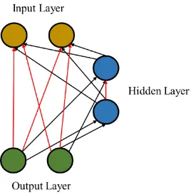
The back propagation artificial neural network (BPANN) is the most commonly used one in Geodesy (Zaletnyik, 2004; Maria, 2012; Lei, Qi, 2010; Tierra and Romero, 2014; Ziggah et al., 2016). This network consists of three types of layers: the input layer, one or more hidden layers and output layer (see Figure 1). The input layer receives the data, whereas the output layer is the last layer that gives the results of the computation. The hidden layer, which is situated between the input and output layers, analyses and processes the data transmitted from the input layer. The number of hidden layers and neurons in the hidden layer may change depending on the problem. In this study, the optimum number of neurons in the hidden layer was obtained by a The International Archives of the Photogrammetry, Remote Sensing and Spatial Information Sciences, Volume XLII-2/W1, 2016
3rd International GeoAdvances Workshop, 16–17 October 2016, Istanbul, Turkey
This contribution has been peer-reviewed.
sequential trial-and-error procedure. The hyperbolic tangent activation function was selected for the hidden layer, while a linear function was selected for the output layer. The training process is based on the delta rule which is used for BPANN training procedure (Haykin, 1999). According to the training algorithms, the weights among the layers are recalculated until the difference between the actual and estimated output values gives small enough values.
Figure 1. Feed forward back propagation network.
The Cascade forward back propagation network is similar to the feed forward networks, but include a weight connection from the input to each layer and from each layer to the successive layers (see Figure 2). While two-layer feed forward networks can potentially learn virtually any input-output relationship, feed-forward networks with more layers might learn complex relationships more quickly. For example, a three-layer network has connections from layer 1 to layer 2, layer 2 to layer 3, and layer 1 to layer 3. The three-layer network also has connections from the input to all three layers. The additional connections might improve the speed at which the network learns the desired relationship. The CFBP and FFBP networks use the back propagation algorithm to update the weights. The main drawback of the CFBP network is that each neuron in this network is related to all previous layer neurons (Beale et al., 2012).
Figure 2. Cascade forward back propagation network.
2.2 Radial Basis Function Neural Network (RBFNN)
The RBFNN is a feed forward network that contains an input layer, a single hidden layer and output layer (see Figure 3). The input layer transmits the inputs to the hidden layer when there are no weights between the hidden and output layers. The hidden layer contains the radial basis functions. Each hidden neuron has its own centroid, and for each input (x1, x2,…, xn), it computes the distance between x and its centroid. Its output is some nonlinear function of that distance. Thus, each neuron in the hidden layer computes an output that depends on a radially symmetric function. The strongest output is generally obtained when the input data is close to the centroid of the node (Park and Sandberg, 1991). Gaussian functions are the most commonly used basis functions of the RBFNNs. The output layer determines the ordinary weighted sum of the output of the hidden neurons. The RBFNN trains faster, compared to other network types. Training of the RBFNNs consists of two stages. In the first stage, the parameters of the hidden neurons (the spread and centre of the radial basis functions) are determined. In the second stage, the weights of the output layer are calculated by means of a supervised training method (Sharaf et. al., 2005).
Figure 3. A RBFNN model with one output.
3. RESULTS
In this paper, 2D coordinate transformation was performed between the ED50 and ITRF96 coordinate systems by using the FFBP, CFBP and RBFNN. Study area is in the city of Trabzon, Turkey. Location of the study area can be seen in Figure 4.
Figure 4. Location of the study area in Turkey.
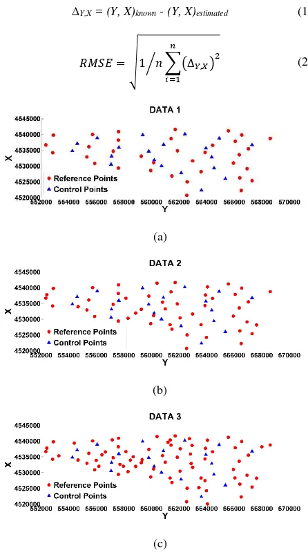
Points with known coordinates were divided into three data sets in both systems. The first data set (Data 1) includes 35 reference points and 20 control points (Figure 5a). The second data set (Data 2) contains 55 reference points and 20 control points The International Archives of the Photogrammetry, Remote Sensing and Spatial Information Sciences, Volume XLII-2/W1, 2016
3rd International GeoAdvances Workshop, 16–17 October 2016, Istanbul, Turkey
This contribution has been peer-reviewed.
(Figure 5b). The third data set (Data 3) includes 74 reference points and 20 control points (Figure 5c).
Performances of the transformation methods were investigated with respect to the root mean square values obtained from the differences between the known coordinates and coordinates estimated by the FFBP, CFBP and RBFNN. RMSE is calculated as;
∆Y,X = (Y, X)known - (Y, X)estimated (1)
� � = √1 � ∑(∆ , ) �
�=
⁄ (2)
(a)
(b)
(c)
Figure 5. The distribution of reference and control points at the study area: (a) Data 1, (b) Data 2, (c) Data 3.
An artificial neural network script was written with the MATLAB ANN toolbox to test the used algorithms. During the training process of the neural networks, the input layer contained YED50 and XED50 coordinates of the reference points, while the output layer contained YITRF96 and XITRF96 coordinates of the reference points. The number of neurons in the hidden layer was specified with a sequential trial-and-error procedure. The hyperbolic tangent sigmoid and linear functions were used as the activation functions of the hidden and output nodes, respectively for the FFBP and CFBP. The Bayesian Regulation optimization technique was used to train these networks. Also, the Gaussian transfer function was used for the hidden layer of the RBFNN. The statistics calculated for each ANN method are given in Table 1.
Table 1. Performance statistics calculated using FFBP, CFBP and RBFNN methods for reference and control points in Y and X directions (units: cm).
Data Set
ANN Type
ΔY
RMSE Train
ΔX
RMSE Train
ΔY
RMSE Test
ΔX
RMSE Test
Data1 FFBP
2:19:2 0.85 0.90 1.40 1.27
Data 1 CFBP
2:24:2 0.80 0.78 1.26 1.18
Data 1 RBFNN
2:20:2 0.68 0.70 1.54 1.09
Data 2 FFBP
2:14:2 1.06 1.40 1.26 1.21
Data 2 CFBP
2:11:2 1.00 0.81 1.74 1.18
Data 2 RBFNN
2:19:2 0.95 0.71 1.48 1.03
Data 3 FFBP
2:26:2 1.02 0.94 1.29 1.09
Data 3 CFBP
2:12:2 1.03 0.96 1.41 0.97
Data 3 RBFNN
2:21:2 1.03 0.94 1.38 1.02
Figure 6 shows the RMSE values calculated using FFBF, CFBP and RBFNN algorithms for control points in Y and X directions.
Figure 6. Graphical representation of the performance statistics calculated using FFBP, CFBP and RBFNN methods in control
points.
4. CONCLUSION
Artificial neural network applications have been widely used in geodetic science. The objective of this paper was to examine 2D coordinate transformation issue between the ED50 and ITRF96 systems by using the FFBP, CFBP and RBFNN artificial neural network algorithms. As seen in Table 1, for Y direction, ±1.26cm (for Data 1), ±1.26cm (for Data 2) and ±1.29cm (for Data 3) RMSEs were obtained with the CFBP, FFBP and FFBP, respectively. For X direction, ±1.09cm (for Data 1), ±1.03cm (for Data 2) and ±0.97cm (for Data 3) RMSEs were obtained with the RBFNN, RBFNN and CFBP, respectively. It was also concluded that the variability among the number of points in data sets did not cause a significant change. The main conclusion drawn from this study is that the ANN algorithms can be used for 2D coordinate transformation in cases where optimum model The International Archives of the Photogrammetry, Remote Sensing and Spatial Information Sciences, Volume XLII-2/W1, 2016
3rd International GeoAdvances Workshop, 16–17 October 2016, Istanbul, Turkey
This contribution has been peer-reviewed.
parameters are selected. A similar study may be conducted by using different ANN models and coordinate systems.
REFERENCES
AL-Allaf, O., N. A., 2012. Cascade-forward vs. function fitting neural network for improving image quality and learning time in image compression system. In Proceedings of the world congress on engineering. 2, pp. 4-6.
Bao, H., Zhao, D., Fu, Z., Zhu, J. and Gao, Z., 2011. Application of genetic-algorithm improved BP Neural Network in automated deformation monitoring," Natural Computation (ICNC), 2011 Seventh International Conference on, Shanghai, pp. 743-746.
Beale, M. H., Hagan, M. T. and Demuth, H. B., 2012. Neural network toolbox™ user’s guide. In R2012a, The MathWorks, Inc., 3 Apple Hill Drive Natick, MA 01760-2098, www. mathworks. com.
Chen, H. and Zeng, Z., 2013. Deformation prediction of landslide based on improved back-propagation neural network. Cognitive computation, 5(1), pp. 56-62.
Du, S., Zhang, J., Deng, Z. and Li, J., 2014. A Neural Network based Intelligent Method for Mine Slope Surface Deformation Prediction Considering the Meteorological Factors. Indonesian Journal of Electrical Engineering and Computer Science, 12(4), pp. 2882-2889.
Gao, C. Y., Cui, X. M. and Hong, X. Q., 2014. Study on the Applications of Neural Networks for Processing Deformation Monitoring Data. Applied Mechanics and Materials. Vol. 501, pp. 2149-2153.
Ghilani, C. D., 2010. Adjustment computations: spatial data analysis. John Wiley & Sons.
Gullu, M., 2010. Coordinate transformation by radial basis function neural network. Scientific Research and Essays, 5(20), pp. 3141-3146.
Gullu, M., Yilmaz, M., Yilmaz, I. and Turgut, B., 2011. Datum Transformation by Artificial Neural Networks for Geographic Information Systems Applications. In International Symposium on Environmental Protection and Planning: Geographic Information Systems and Remote Sensing Applications, pp. 28-29.
Haykin, S., 1999. Neural Networks A Comprehensive Foundation, 2nd Edition, Prentice Hall Publishing, New Jersey, USA.
Hai, T. S. and Thuy, N. T., 2012. Image classification using support vector machine and artificial neural network. International Journal of Information Technology and Computer Science (IJITCS), 4(5), pp. 32-38.
Ibrahim, F. B,. 2010. Image compression using multilayer feed forward artificial neural network and dct. Journal of Applied Sciences Research, 6(10), pp.1554-1560.
Kavzoglu, T. and Saka, M. H., 2005. Modelling local GPS/levelling geoid undulations using artificial neural networks. Journal of Geodesy, 78(9), pp. 520-527.
Liao, D. C., Wang, Q. J., Zhou, Y. H., Liao, X. H. and Huang, C. L., 2012. Long-term prediction of the Earth Orientation Parameters by the artificial neural network technique. Journal of Geodynamics, 62, pp. 87-92.
Weiwei, L. and Xiudong, Q., 2010. The Application of BP Neural Network in GPS Elevation Fitting, Intelligent Computation
Technology and Automation (ICICTA), 2010 International Conference, Changsha, pp. 698-701.
Memarian Sorkhabi, O., 2015. Geoid Determination Based on Log Sigmoid Function of Artificial Neural Networks:(A case Study: Iran). Journal of Artificial Intelligence in Electrical Engineering, 3(12), pp. 18-24.
Maria, M. F. R., 2012. Coordinate transformation for integrating map information in the new geocentric European system using Artificial Neural Networks. GeoCAD, pp. 1-9.
Pikridas, C., Fotiou, A., Katsougiannopoulos, S. and Rossikopoulos, D., 2011. Estimation and evaluation of GPS geoid heights using an artificial neural network model. Applied Geomatics, 3(3), pp. 183-187.
Schuh, H., Ulrich, M., Egger, D., Müller, J. and Schwegmann, W., 2002. Prediction of Earth orientation parameters by artificial neural networks. Journal of Geodesy, 76(5), pp. 247-258.
Sharaf, R., Noureldin A., Osman, A. and EI-Sheimy, N., 2005. Online INS/GPS integration with a radial basis function neural network, IEEE Aerospace and Electronic Systems Magazine. 20(3), pp. 8-14.
Tierra, A., Dalazoana, R. and De Freitas, S., 2008. Using an artificial neural network to improve the transformation of coordinates between classical geodetic reference frames. Computers & Geosciences, 34(3), pp. 181-189.
Tierra, A. and Romero, R., 2014. Planes coordinates transformation between PSAD56 to SIRGAS using a Multilayer Artificial Neural Network. Geodesy and Cartography, 63(2), pp. 199-209.
Zaletnyik, P., 2004. Coordinate transformation with neural networks and with polynomials in Hungary. In Proceedings of International Symposium on Modern Technologies, Education and Professional Practice in Geodesy and Related Fields, Sofia, Bulgaria, pp. 471-479.
Ziggah, Y. Y., Youjian, H., Yu, X. and Basommi, L. P., 2016. Capability of Artificial Neural Network for Forward Conversion of Geodetic Coordinates (ϕ, λ, h) to Cartesian Coordinates (X, Y, Z). Mathematical Geosciences, 48(6), pp. 687-721.
The International Archives of the Photogrammetry, Remote Sensing and Spatial Information Sciences, Volume XLII-2/W1, 2016 3rd International GeoAdvances Workshop, 16–17 October 2016, Istanbul, Turkey
This contribution has been peer-reviewed.