LOCALIZATION USING RGB-D CAMERAS ORTHOIMAGES
Marie-Anne MITTET, Tania LANDES, Pierre GRUSSENMEYER
ICube Laboratory UMR 7357, Photogrammetry and Geomatics Group, INSA Strasbourg, France (marie-anne.mittet, tania.landes, pierre.grussenmeyer)@insa-strasbourg.fr
Commission 5WG V, ICWG I/Va
KEY WORDS:mobile mapping, system, orthoimage, urban environment, range imaging camera
ABSTRACT:
3D cameras are a new generation of sensors more and more used in geomatics. The main advantages of 3D cameras are their handiness, their price, and the ability to produce range images or point clouds in real-time. They are used in many areas and the use of this kind of sensors has grown especially as the Kinect (Microsoft) arrived on the market. This paper presents a new localization system based exclusively on the combination of several 3D cameras on a mobile platform. It is planed that the platform moves on sidewalks, acquires the environment and enables the determination of most appropriate routes for disabled persons. The paper will present the key features of our approach as well as promising solutions for the challenging task of localization based on 3D-cameras. We give examples of mobile trajectory estimated exclusively from 3D cameras acquisitions. We evaluate the accuracy of the calculated trajectory, thanks to a reference trajectory obtained by a total station.
1. INTRODUCTION AND RELATED WORK
The development of the system presented in this paper meets the needs of a current R&D project Terra Mobilita, gathering 8 partners from industry and public institutions (STAR APIC, THALES TRAINING SYSTEM, MENSI-TRIMBLE, DRYADE, IGN, ARMINES, Sciences Po Foundation, CEREMH). The aim of the Terra Mobilita project is to develop new automatic pro-cesses for 3D urban maps creation and updates based on new mobile laserscanning techniques. It is planned that the platform moves on sidewalks, acquires the environment and enables the determination of most appropriate routes for disabled persons with centimeter accuracy (http://www.terramobilita.fr). In urban environments, the use of classical localization solutions like GNSS is limited to areas providing sufficient satellite visibility. In this context, a localization system supported exclusively by 3D cam-eras has been proposed.
3D cameras have several advantages, including their usability and their ability to produce depth images or point clouds in real time. They are used for many applications, such as user interaction (gesture recognition) as mentioned in (Kolb et al., 2008), pattern recognition (Kolb et al., 2009) or scene analysis in robotics (May et al., 2006).
The marketing of the Microsoft Kinect in 2010 and of the Asus Xtion Pro in 2011, both based on the technology developed by PrimeSense (Arieli et al., 2010), led to the wide dissemination of this kind of sensors. Every 40 millisecond, these sensors provide depth images of 640 x 480 pixels, from which point clouds can be generated.
For guarantying the reliability of the point clouds, especially with the purpose of precise localization, a prior calibration must be carried out. More information about 3D camera calibration can be found in (Mittet et al., 2013).
When excluding GNSS solutions, the localization of a mobile platform requires the estimation of its position over time using the information it acquires about the environment around him. The operation consisting in defining the displacement performed by a moving object (vehicle, wheeled robots or legged robots) based on the data collected by its actuators, is called odometry.
In the case of a wheeled object, the actuators are rotary encoders. In the case of system exclusively based on cameras, odometry is performed using the images they collect. The terminology vi-sual odometry has been introduced by (Nist´er et al., 2004). It consists in defining the displacement of the mobile based on the detection of the changes between successive images taken by the cameras on board. The main advantage of visual odometry com-pared to classical odometry is that it is not sensitive to terrain turbances. Indeed, rotary encoders usually provide a biased dis-tance when the platform crosses sidewalks (loss of contact with the ground). Moreover, since visual odometry is based on images, it gives the opportunity to take benefit from well-known image processing tools. Visual odometry is largely mentioned in the literature ((Nist´er et al., 2004), (Maimone et al., 2007), (Fraun-dorfer and Scaramuzza, 2012)). The main processing steps are feature detection, feature matching (or tracking) and motion esti-mation (Scaramuzza and Fraundorfer, 2011). Since visual odom-etry is performed on images, it can be applied on several camera systems, like monocular cameras (Kitt et al., 2011), stereo-vision systems (Nist´er et al., 2004); (Howard, 2008), omnidirectional cameras (Scaramuzza and Siegwart, 2008) and more recently 3D cameras (Huang et al., 2011).
Section 2 presents the developed 3D camera system. Not only the configuration but also the visual odometry approach is de-tailed. The originality of the localization approach comes from the use of previously generated orthoimages. The most frequently feature detectors encountered in the literature are compared and assessed. Then a feature tracking step enables the displacement estimation. Section 3 evaluates the quality of the computed tra-jectory provided by the localization approach. Finally solutions for improving the system are suggested.
2. DEVELOPED APPROACH
2.1 System presentation
meets the following requirements: maximal ground coverage in the motion direction and reduced overlapping areas. Indeed, given the technology used by Kinect, it is to expect that overlapping ar-eas induce mar-easurement artefacts. In order to cover a wider field of view, three cameras have been installed on the platform. They have been tilted in order to bring the field of view border as close as possible to the vehicle. The position and orientation of the 3 cameras enable to cover about 9 x 6 meters area in front of the platform. After creative design study, the final prototype has been conceived in CAD environment (Figure 1) and constructed as shown in Figure 2.
Figure 1: CAD model Figure 2: Prototype
2.2 About the creation and use of orthoimages
This section presents the calibration performed on our system to merge the captured clouds. Then, the generation of orthoimages, based on merged point clouds, is exposed. These orthoimages are then used to estimate the displacement of our mobile.
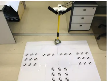
2.2.1 Point cloud generation One camera (Asus Xtion Pro) produces a point cloud composed of 300000 points. For process-ing the information of the three point clouds captured by the three cameras, a fusion of the point clouds is suggested. This step re-quires the knowledge of the 3D relative transformations between the frames of the cameras. For determining them, a pattern of targets has been constructed (Figure 3). The targets coordinates are measured in the three point clouds and matched with their co-ordinates on the pattern. At this stage, it is possible to calculate the translations and rotations between the 3 cameras (Table 1).
Figure 3: Calibration sheet
2.2.2 Orthoimage generation After fusion of the point clouds of the three cameras, the system is able to produce point clouds of 900000 points for one position of the platform. Obviously, the dataset might become voluminous and consequently the process is time consuming. That is why, instead of operating in 3D point clouds, we decided to orthoproject the points onto the ground.
Camera 1 Camera 2 Camera 3
Ω 16.7186 39.3136 13.7818
(±0.2353) (±0.1405) (±0.2319)
Φ 36.1954 -2.2857 -37.2252
(±0.2413) (±0.1826) (±0.3102)
κ -29.5936 -93.7636 -158.8719 (±0.2054) (±0.1634) (±0.2216)
Tx 0.656 m 0.580 m 0.517
(±0.003) (±0.003) (±0.004 )
Ty 0.792 m 0.768 m 0.837 m
(±0.003) (±0.002) (±0.003)
Tz -0.618 m -0.615 m -0.605 m (±0.003) (±0.002) (0.003)
Table 1: Coordinates of each camera in the frame of the calibra-tion sheet. Ω,Φ,κare the rotation angles, andTx, Ty,Tzthe translation.
This idea has several advantages. Firstly, the well-known 2D al-gorithms which have proven their efficiency in the image process-ing field can be applied on these orthoimages. Secondly, an or-thoimage simplifies drastically the 3D environment without los-ing the altimetric information.
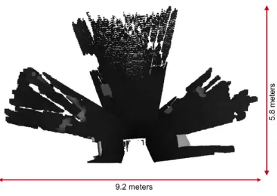
In order to create an orthoimage, it is necessary to calculate the ground pixel size covered by a point of the point cloud. Asus Xtion Pro provides depth images of 640 x 480 pixels. From this depth image, it is possible to generate a point cloud. Given the acquisition geometry shown in Figure 4 and knowing the height (h) of the camera and its orientation to the ground (θ), the part covered by the pixel on the ground can be calculated using equa-tion (1). It must be denoted that the size of the pixels grows with the range. The pixels of the orthoimage are coded in grayscale regarding the point altitude. Therefore the third dimension infor-mation is kept. An example of orthoimage is presented in Fig-ure 5.
Figure 4: System geometry
∆y= p
h2+y2.tan∆θ
Figure 5: Orthoimage obtained from our system
Our localization approach is based on the determination of the mobile displacement observed between orthoimages acquired reg-ularly during the movement. The presented system produces, for each timet, one point cloud of 900000 points. This point cloud is transformed into an orthoimage calledOt. The set of orthoimages is denotedO0:n = O0, ..., On. The determination of the platforms trajectory requires computing the displacement performed between two successive orthoimages. This displace-ment is obtained through the calculation of the transformations parametersTt,t−1between the orthoimageOtat timetand the orthoimageOt−1att−1. At timet, the position of the platform
is defined by equation 2.
Pt=Pt−1∗Tt,t−1(withP0=I) (2)
In previous equation, the rigid transformationTt,t−1is defined as
detailed in equation (3).
whereRt,t−1∈SO(3)(3D rotation group) is the rotation matrix,
andtt,t−1∈R 3×1
is the translation vector.
The positionPn of the camera system is obtained by concate-nating all transformationsTt (t = 1...n). Therefore we have
Pn = Pn−1Tn,n−1. The initial position is given byP0 at tilt
t= 0, initialised as the user wishes. The whole positions occu-pied by the system is thereforeP0:n={P0, ..., Pn}.
2.3 Features extraction and tracking
In our approach, visual odometry is based on the estimation of displacements occurred between two successive orthoimages. The transformation calculation requires firstly the detection of corre-sponding points in two successive orthoimages. For every image to process at timet, firstly the feature points are detected and then their homologous points in the orthoimage taken att−1
are searched. The feature extraction step as well as the following matching step are crucial because their robustness and rapidity in-fluence the trajectory accuracy and the trajectory calculation time.
In this context, several detectors and descriptors have been com-pared and assessed. Among the mostly used and well-known
detectors, there are corners detectors like (Harris and Stephens, 1988) or GFTT from (Shi and Tomasi, 1994) and blob detec-tors like SIFT (Lowe, 2004), SURF (Bay et al., 2006) or ORB (Rublee et al., 2011). SIFT, SURF and ORB are widely used in visual localization. They look for regions with invariance proper-ties including invariance to scaling and rotations.
The SIFT detector, although it is already ten years old, has proven its superiority in many applications related to points of interest (features). However, it suffers from computational complexity making it too slow for real-time applications such as SLAM or visual odometry. Faced with this problem, many improvements have been performed on the SIFT detection algorithm. Our study will focus on one of the most famous of them, SURF, and a more recent detector, ORB, which is itself a derivative of FAST (Ros-ten and Drummond, 2006). The approach proposed by (Shi and Tomasi, 1994) will also be taken into account in this study, be-cause this detector is known for its effectiveness in visual odom-etry applications ((Nist´er et al., 2006), (Milella and Siegwart, 2006)).
2.3.1 Assessment of features detectors The motion estima-tion is carried out using the points detected in the orthoimages. Detection of landmarks plays a fundamental role in the overall functioning of our system. This step can be computationally ex-pensive, and thus the speed of localization will depend directly on the speed of detection. It is also noted that the accuracy of de-tection, i.e. the ability to ”re-discover” the same points in two successive orthoimages will affect the accuracy of the motion estimation. Finally, the number of points detected and mapped should be sufficient to find the transformation between two or-thoimages. In order to find the most suitable detector for our application, different criteria are taken into account :
• the stability of the detector,
• the number of detected features,
• and finally the detection time.
(Mikolajczyk and Schmid, 2005) propose a method for assessing detectors. Stability of the detectors is evaluated using the crite-rion of repeatability. The repeatability rating for a pair of cor-responding images is computed as the ratio between the correct correspondences, and the total number of detected points (equa-tion 3). The same points detected in two images are appointed as correspondences. Knowing the transformation between two images, these correspondences are computed by applying the in-verse transform to the points of the second image. If locally the region around this point has sufficient overlap with the corre-sponding point in the first image, then it is considered as a good correspondence. Thus, if two images contain respectivelyn1and
n2detected points, then the repeatability criterion is defined as follows :
repeatability=good correspondances
min(n1, n2)
(4)
The repeatability criterion is a good estimator to evaluate the sta-bility of the detectors. As seen previously, this property has an impact on the final precision of our application, therefore it is im-portant to study this criterion.
point clouds can be generated with Blensor (Gschwandtner et al., 2011). Blensor is an application which permits the 3D modeling of scenes, and the simulation of 3D data as acquired by systems such as LIDAR, ToF cameras, as well as 3D cameras. It allows the definition of a 3D scene within Blender, and afterwards the acquisition of a sensor by placing it in this scene (Figure 6). It is equally possible to define a displacement to be followed by the sensor in the scene. Therefore, the user can ask the sensor to follow a specific trajectory. Based on this known trajectory, the transformation between to successive point clouds (and therefore orthoimages) is known.
(a) (b)
Figure 6: Image used in order to assess features detectors a) 3D scene used to generate the orthoimage ; b) Orthoimage obtained thanks to the 3D scene (simulated data)
Based on these images, the repeatability criterion of Shi-Tomasi, SIFT, SURF and ORB detectors has been calculated. The evalu-ations were performed for rotevalu-ations and translevalu-ations transforma-tions.
Figure 7: Repeatability of detector for several rota-tion angles
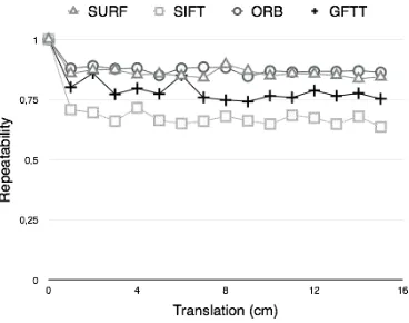
As presented in Figure 7, for low rotations, ORB and SURF have a better repeatability than other detectors. However, when the ro-tation angle increases, SURF presents better results. Also in the case of translation, ORB and SURF stand out (Figure 8).
The second criterion covered by our study is the number of tected points. As presented in Table 2, the largest number of de-tected points is provided by ORB, and the lowest by SIFT.
SURF SIFT ORB GFTT
Number of detected points 612 500 1271 1255
Table 2: Number of detected points, based on the orthoimage of Figure 6b
The third criterion on which our study is focused concerns the detection time. Indeed, the final application aims to operate in
Figure 8: Repeatability of the detectors for several translations
real time, so it is necessary to choose an efficient detector not only in terms of precision, but also in terms of speed. That’s why the ratiodetection time/nb pointhas been studied (Figure 9).
Figure 9: Execution time for different detectors (in seconds)
As illustred in Figure 9, from a temporal point of view, ORB and GFTT are faster than SURF. SIFT is the slowest among the eval-uated detectors.
On the basis of the three selected criteria, namely the repeata-bility, the number of detected points and the speed, we were able to determine the most appropriate detector for our approach. As regards to the criterion of repeatability, ORB has the best results both for rotational movements and for linear movements. Re-garding the number of detected points, it is also ORB that pro-vides most of points of interest. Finally, from a temporal point of view, it is still ORB that provides the most satisfying results. In conclusion, ORB provides the best results and has been adopted in the implementation of our approach.
2.3.2 Matching or tracking ? Once this detection step is ma-de, it is necessary to connect the detected points between two suc-cessive orthoimages. There are two approaches to achieve this stage : matching and tracking. The matching operates in four steps. Firstly, it detects points of interest in two images. Then, detected points are associated with their descriptors. The descrip-tors are compared using a similarity measure. After comparing descriptors of the first image with the descriptors of the second image, the best correspondence between two points of interest is selected by the nearest descriptor. Symmetrical correspondences are considered as more reliable than asymetrical ones.
Figure 10 shows the 3D scene used to generate orthoimages in order to compare tracking and matching. Figure 11a presents the results of correspondences obtained for tracking and Figure 11b presents the results of correspondences obtained for matching. This experiments shows that, given the type of images we treat (orthoimages), it seems more appropriate to use an approach based on tracking. In fact, the orthoimages used are highly uniform.
In this context, we decided to developed an algorithm based on the approach proposed by (Lucas and Kanade, 1981) and im-proved with the pyramidal implementation (Bouguet, 2001). This allows us to perform the tracking of points even in the case of large displacements between two images.
Despite the use of tracking, bad correspondences remain in the dataset. It is then necessary to remove them in order to calcu-late the most accurate motion estimation. In the next section we propose to introduce the method implemented to eliminate outlier correspondences.
Figure 10: 3D scene used to generate the orthoimage in order to compare tracking and matching approaches
(a) (b)
Figure 11: Correspondences obtained for : a) tracking ; and b) matching. The vectors in green represent the calculated corre-spondences
2.4 Outliers removal
When it is needed to estimate a model, it is always necessary to remove outliers, in our case the bad correspondences. The sample consensus RANSAC (Fischler and Bolles, 1981) is a classical ap-proach for model estimation in the presence of outliers. Structure from motion (SFM) is one of the applications of RANSAC. In the case of SFM, the model to discover is a movement composed of a translation and a rotation(R, t). The principle of RANSAC is based on calculating an hypothesis from a subset chosen ran-domly from the original sample, and to verify this hypothesis with the rest of the data. The hypothesis which has the highest consen-sus is considered as being the best solution. The number of iter-ationsN necessary to obtain a solution is computed in equation 5.
wheresis the number of minimal data points,ǫis the percentage of outliers in the data points, andpis the requested probability of
N= log(1−p)
log(1−(1−ǫ)s) (5)
success (Fischler and Bolles, 1981).Ngrows exponentially with the number of points necessary for estimating the model. There is a great interest in finding the minimal parametrization of the model because N might slow down the motion estima-tion algorithm. For a movement without constraints (6 degrees of freedom) from a calibrated camera, it is necessary to have 5 correspondences. In the case of a planar motion, the model com-plexity is reduced to 3 DoF and can be estimated with 2 points as described in (Ortin and Montiel, 2001).
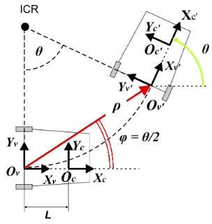
In (Scaramuzza, 2011), the author suggests to exploit the non holonomic constraint of the vehicle on which the acquisition sys-tem is placed. This configuration permits to use a restrictive mo-tion model which allows to parameterize the momo-tion with only one correspondence. When a wheeled vehicle rotates around a point, the trajectory described by each wheel is a circle. The cen-ter of this circle is called Instantaneous Cencen-ter of Rotation (ICR) in Figure 12. ICR can be computed by intersecting all the roll axes of the wheels. This property can be applied to mobiles as car or robots, or to our mobile. Let us assume the camera system is fixed somewhere on our mobile (with origin inOc), as depicted in Figure 12. In the orthoimage frame corresponding to this po-sition, the axisZcis orthogonal to the plane of motion, andXc is oriented perpendicularly to the back wheel axis of the mobile. After a displacement of the mobile, we can then defineOc′ the origin, andZc′,Xc′the axis of the reference of our mobile. The movement of a camera mounted on the mobile can be locally de-scribed as a circular displacement. This reduces the movement to only two degrees of freedom, namely the angle of rotation (θ), and the radius of curvature (in the case of a translation, the radius of curvature tends to infinity). Every feature correspondence can be named ”vector of displacement”, and defined by two parame-ters,θandρ.
Figure 12: Circular motion of a wheeled vehicle (Scara-muzza, 2011)
It is then possible to calculateθfor each of these vectors. Conse-quently, RANSAC can be initialised with only one correspon-dence. As an alternative, the author also suggests to use his-togram voting. Indeed, it is possible to construct an hishis-togram ofθvalues, where each bin represents the number of correspon-dences having the sameθ.
The vector of correspondence should provide the same value for
13 presents the histogram obtained for theθcalculations related to Figure 11a.
This approach is not iterative, thus it greatly simplifies the com-putational complexity of this step. Furthermore the quality of inliers is not equivalent in the entire image. As mentioned in the section explaining the orthoimages generation (section 2.2.2,) the most distant points will be less accurate. This means that, de-pending on the distribution of correspondences in the scene, the inliers found by RANSAC might be different, and therefore might affect the final motion estimation.
Figure 13: Histogram obtained for theθcalculation related to Figure 11a
In summary, the overall motion estimation algorithm developed in our work is divided in five steps :
1. Generation of an orthoimage from the current point cloud
2. Extraction of feature correspondences between current and previous orthoimages
3. Calculation of the pixel distance between the corresponding points. If more than 90% of the distances are less than 3 pixels then assume no motion and return to step 1
4. Removing the outliers using histogram voting
5. Calculation of the motion estimation from all the remaining inliers.
It must be denoted that the previous poses and structure are not used to refine the current estimate.
3. QUANTITATIVE ASSESSMENT OF OUR APPROACH
In order to validate the developed approach, a dataset has been acquired in laboratory conditions. The mobile platform (Fig-ure 14a) has been pushed on about 20 meters in a large room. Several objects have been integrated to the scene for simulating urban furniture (Figure 14b).
The acquisition has been performed inside a building, because currently the Kinect technology remains inefficient outside (ex-cept during sunless days). To evaluate the accuracy of the calcu-lated trajectory, a reference trajectory is needed. In fact, during its displacement, the mobile platform has been tracked simulta-neously by total station measurements. Therefore, the deviations between the calculated trajectory and the reference trajectory pro-vide a quantitative assessment of the localization algorithm.
3.1 Results
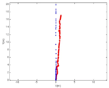
During this acquisition, 1400 point clouds were saved and merged, and 1400 orthoimages have been produced. The estimated path is indicated in red dots in Figure 15 and the path obtained through
(a) (b)
Figure 14: Mobile platform (a) and acquisition scene, with in red the path followed by our mobile system (b)
the total station is indicated in blue dots. The final drift at the end is about 1.3 m after 20 meters of displacement. It is observed that the drift is constant during the movement. This result is already quite good if one considers that the proposed approach is incre-mental (at each new orthoimage only the current pose is updated without refining the previous poses).
Figure 15: Comparison between estimated path (in red) and path obtained via total station (in blue)
3.2 Limitations
The assessment of the computed trajectory has highlighted some limitations regarding our system.
Firstly the position of the 3 cameras introduces a discontinuity in the global field of view of the system, because the three fields of view are not overlapping (Figure 5). This causes errors in the transformation calculation especially when objects are lost by the detection process as soon as they enter into these empty areas.
ranges are given in millimeters and fixed, the distance informa-tion may change from one interval to another. Therefore the dif-ference between two successive point clouds even if the mobile is stationary introduces errors in the trajectory calculation. It is then necessary to filter this phenomenon, but it remains difficult to distinguish between a real displacement, and a displacement due to measurement noise.
3.3 Solutions
Several solutions are proposed to solve these problems. On the one hand, we plan to take advantage from the objects shadows moving between two successive frames. On the other hand, it seems interesting to label encountered objects as individual en-tities. Finally, this evaluation showed the necessity to assign a memory to the detection algorithm. It means that every object oc-curring in the scene must be recorded and followed. This memory assignment is essential for detecting the points encountered twice in a pass, like in the case of a loop closure. A global optimiza-tion procedure in which weights will be assigned to the detected features is also under progress.
4. CONCLUSION AND PERSPECTIVES
In this paper, we describe a new localization system for estimat-ing the relative displacement of a mobile plateform. This local-ization system is composed of RGB-D cameras exclusively. It should be noted that our algorithm is system independent. All of our developments have been implemented in order to be valid for any type of 3D camera. From our system it is possible to ob-tain orthoimages computed from point cloud provided by RGB-D cameras. We also present our algorithm, which permits us to compute the motion estimation of our plateform. The proposed approach was applied to real data, and the quantitative assesse-ment was realized by comparing our result to the real position of the platform obtained by total station measurements. Further-more, in the near future, we plan to improve our approach by in-tegrating a memory as well as bundle block adjustment process.
REFERENCES
Arieli, Y., Freedman, B., Machline, M. and Shpunt, A., 2010. Depth mapping using projected patterns - Patent nb : US20080240502.
Bay, H., Tuytelaars, T. and Gool, L. V., 2006. Surf: Speeded up robust features. In: Proceedings of the European Conference on Computer Vision, pp. 404–417.
Bouguet, J. Y., 2001. Pyramidal Implementation of the Lucas Kanade Feature Tracker Description of the algorithm. Technical report, OpenCV Document, Intel Microprocessor Research Labs.
Fischler, M. A. and Bolles, R. C., 1981. Random sample consen-sus: a paradigm for model fitting with applications to image anal-ysis and automated cartography. Communications of the ACM 24(6), pp. 381–395.
Fraundorfer, F. and Scaramuzza, D., 2012. Visual Odometry : Part II - Matching, Robustness, and Applications. Robotics & Automation Magazine, IEEE 19(2), pp. 78–90.
Gschwandtner, M., Kwitt, R., Uhl, A. and Pree, W., 2011. Blensor : Blender Sensor Simulation Toolbox. In: Proceedings of 7th International Symposium In Advances in Visual Computing, pp. 199–208.
Harris, C. and Stephens, M., 1988. A combined corner and edge detector. In: Proceedings of the Alvey Vision Conference, Vol. 15, pp. 147–151.
Howard, A., 2008. Real-time stereo visual odometry for au-tonomous ground vehicles. Proceedings of Intelligent Robots and Systems, 2008. IEEE/RSJ International Conference. pp. 3946– 3952.
Huang, A. S., Bachrach, A., Henry, P., Krainin, M., Maturana, D., Fox, D. and Roy, N., 2011. Visual Odometry and Mapping for Autonomous Flight Using an RGB-D Camera. In: Proceedings of International Symposium on Robotics Research (ISRR), pp. 1– 16.
Kitt, B. M., Rehder, J., Chambers, A. D., Schonbein, M., Late-gahn, H. and Singh, S., 2011. Monocular visual odometry using a planar road model to solve scale ambiguity. In: Proceedings of European Conference on Mobile Robots.
Kolb, A., Barth, E. and Koch, R., 2008. ToF-Sensors : New Di-mensions for Realism and Interactivity. In: Proceedings of puter Vision and Pattern Recognition Workshops. IEEE Com-puter Society Conference., pp. 1–6.
Kolb, A., Barth, E., Koch, R. and Larsen, R., 2009. Time-of-Flight Sensors in Computer Graphics. In: Proceedings of Euro-graphics (State-of-the-Art Report), Vol. 29, pp. 141–159.
Lowe, D. G., 2004. Distinctive Image Features from Scale-Invariant Keypoints. International Journal of Computer Vision 60(2), pp. 91–110.
Lucas, B. and Kanade, T., 1981. An iterative image registra-tion technique with an applicaregistra-tion to stereo vision. In: IJCAI, pp. 674–679.
Maimone, M., Cheng, Y. and Matthies, L., 2007. Two years of Visual Odometry on the Mars Exploration Rovers. Journal of Field Robotics 24(3), pp. 169–186.
May, S., Surmann, H., Perv, K. and Augustin, D.-S., 2006. 3D time-of-flight cameras for mobile robotics. In: Proceedings of the IEEE/RSJ International Conference on Intelligent Robots and Systems, pp. 790–795.
Mikolajczyk, K. and Schmid, C., 2005. Performance evaluation of local descriptors. Pattern Analysis and Machine Intelligence, IEEE Transactions on 27(10), pp. 1615–1630.
Milella, A. and Siegwart, R., 2006. Stereo-based ego-motion es-timation using pixel tracking and iterative closest point. In: Pro-ceedings of IEEE International Conference on Computer Vision Systems, pp. 21–24.
Mittet, M.-A., Grussenmeyer, P., Landes, T., Yang, Y. and Bernard, N., 2013. Mobile outdoor relative localization using calibrated RGB-D cameras. In: 8th International Symposium on Mobile Mapping Technology, pp. 2–7.
Nist´er, D., Naroditsky, O. and Bergen, J., 2004. Visual odome-try. In: Proceedings of International Conference Computer Vision and Pattern Recognition, Vol. 1, pp. 652–659.
Nist´er, D., Naroditsky, O. and Bergen, J., 2006. Visual odometry for ground vehicle applications. Journal of Field Robotics 23(1), pp. 3–20.
Rosten, E. and Drummond, T., 2006. Machine learning for high-speed corner detection. In: Proceedings of the European Confer-ence on Computer Vision, pp. 430–443.
Rublee, E., Rabaud, V., Konolige, K. and Bradski, G., 2011. ORB: An efficient alternative to SIFT or SURF. In: Proceedings of International Conference on Computer Vision, pp. 2564–2571.
Scaramuzza, D., 2011. 1-Point-RANSAC Structure from Mo-tion for Vehicle-Mounted Cameras by Exploiting Non-holonomic Constraints. International Journal of Computer Vision 95(1), pp. 74–85.
Scaramuzza, D. and Fraundorfer, F., 2011. Visual Odometry: Part I - The First 30 Years and Fundamentals. IEEE Robotics and Automation Magazine 18(4), pp. 80–92.
Scaramuzza, D. and Siegwart, R., 2008. Appearance-Guided Monocular Omnidirectional Visual Odometry for Out-door Ground Vehicles. IEEE Transactions on Robotics 24(5), pp. 1015–1026.