AN ENERGY MINIMIZATION APPROACH TO AUTOMATED EXTRACTION OF
REGULAR BUILDING FOOTPRINTS FROM AIRBORNE LIDAR DATA
Yuxiang He a,b,*, Chunsun Zhang a,c, Clive S. Fraser a,b
a Cooperative Research Centre for Spatial Information, VIC 3053, Australia b Department of Infrastructure Engineering, University of Melbourne, VIC 3010, Australia –
[email protected], [email protected]
c School of Mathematical and Spatial Sciences, RMIT University, VIC 3000, Australia – [email protected]
Commission III, WG III/4
KEY WORDS: Building Footprint, Extraction, LiDAR, Point Cloud, Energy Minimization
ABSTRACT:
This paper presents an automated approach to the extraction of building footprints from airborne LiDAR data based on energy minimization. Automated 3D building reconstruction in complex urban scenes has been a long-standing challenge in photogrammetry and computer vision. Building footprints constitute a fundamental component of a 3D building model and they are useful for a variety of applications. Airborne LiDAR provides large-scale elevation representation of urban scene and as such is an important data source for object reconstruction in spatial information systems. However, LiDAR points on building edges often exhibit a jagged pattern, partially due to either occlusion from neighbouring objects, such as overhanging trees, or to the nature of the data itself, including unavoidable noise and irregular point distributions. The explicit 3D reconstruction may thus result in irregular or incomplete building polygons. In the presented work, a vertex-driven Douglas-Peucker method is developed to generate polygonal hypotheses from points forming initial building outlines. The energy function is adopted to examine and evaluate each hypothesis and the optimal polygon is determined through energy minimization. The energy minimization also plays a key role in bridging gaps, where the building outlines are ambiguous due to insufficient LiDAR points. In formulating the energy function, hard constraints such as parallelism and perpendicularity of building edges are imposed, and local and global adjustments are applied. The developed approach has been extensively tested and evaluated on datasets with varying point cloud density over different terrain types. Results are presented and analysed. The successful reconstruction of building footprints, of varying structural complexity, along with a quantitative assessment employing accurate reference data, demonstrate the practical potential of the proposed approach.
1. INTRODUCTION
Building footprints are important features in spatial information systems and they are used for a variety of applications, such as visual city tourism, urban planning, pollution modelling and disaster management. In cadastral datasets, building footprints are a fundamental component. They not only define a region of interest (ROI), but also reveal valuable information about the general shape of building roofs. Thus, building footprints can be employed as a priori shape estimates in the modelling of more detailed roof structure (Vosselman, 2002).
Remote sensing has been a major data source for building footprint determination and there is ongoing research and development in photogrammetry and computer vision aimed at the provision of more automated and efficient footprint extraction. The sensors employed are generally aerial cameras or LiDAR. Often cited approaches to building footprint determination can be found in Lafarge et al. (2008), Vosselman (1999) and Weidner and Förstner (1995).
The challenge of building footprint extraction from LiDAR data is partially due to either occlusions from neighbouring high objects, such as overhanging trees, or to inherent deficiencies in the LiDAR data itself, such as unavoidable noise and irregular point distribution. As a result, points on building edges usually exhibit a zigzag pattern. To recover regular shape, some methods determine dominant directions from boundary points. Alharthy and Bethel (2002) measured two dominant directions by determining peaks in the histogram of angles. Zhou and
Neumann (2008) extended this work by finding multiple dominant directions from histogram analysis using tangent directions of boundary points. Other methods for determining building shape are based on Mean-shift clustering algorithms (Dorninger and Pfeifer, 2008), minimum bounding rectangles (Arefi and Reinartz, 2013) or generative models (Huang and Sester, 2011). These methods employ a rectilinear prior to regularize polygonal shape. Such an assumption is not appropriate in many cases, especially when buildings exhibit complex structure.
As an alternative strategy, Sester and Neidhart (2008) relied on an explicit representation of boundary shape using a RANSAC method for line segment extraction. The extracted segments provided information on angle transition, which was used to impose constraints of parallelism or perpendicularity. Another strategy, which has also been adopted here, first approximates raw building boundaries as preliminary polygons, and then the outlines are regularized by directional alignment. Kabolizade et al. (2010) improved snake mode for the approximation of initial building boundaries with introducing height and regional similarity. Sampath and Shan (2007) built the preliminary boundary via a Douglas-Peucker (DP) method (Douglas and Peucker, 1973) and the regularized polygon was processed using a rule-based alignment. As suggested in Neidhart and Sester (2008), results from DP approximation can be unsatisfactory because building characteristics are not necessarily retained. Weidner and Förstner (1995) employed a local minimum description length (MDL) approach to simplify the DP result and meanwhile imposed soft constraints to ISPRS Annals of the Photogrammetry, Remote Sensing and Spatial Information Sciences, Volume II-3, 2014
regularize polygonal shape. A similar approach can be found in Jwa et al. (2008) where MDL was extended by adding a global directional constraint. Wang et al. (2006) also followed this general workflow for preliminary boundary extraction, leading to a new regularization method where the building footprint is determined by maximizing the posterior expected value. The prior was formulated as the belief in the likelihood of various hypotheses and the fitting error was employed to encode the probability of boundary points belonging to a particular building footprint model.
This paper presents a novel approach, based on energy minimization, to simplifying and refining building footprints from LiDAR data. A primary focus of the paper is on the adoption of energy minimization to determine the optimal hypothesis of polygons derived from a vertex-driven DP method and to infer the best connection structure in areas where the building outlines are ambiguous due to insufficient LiDAR point coverage. A global adjustment is conducted to enforce geometric building footprint properties, such as parallelism and perpendicularity.
The rest of this paper is structured as follows: Section 2 briefly introduces the principle of energy minimization and its application in photogrammetry and computer vision. Section 3 then presents the vertex-driven DP method and the energy minimization is used to select the optimal hypothesis. In Section 4, hybrid reconstruction in terms of explicit and implicit modelling through energy minimization is described in detail. Results are illustrated in Section 5 to demonstrate the potential of the proposed approach. Conclusions are offered in Section 6.
2. ENERGY MINIMIZATION
Energy minimization is an expressive and elegant framework to alleviate uncertainties in sensor data processes and ambiguities in solution selection (Boykov et al., 1999). It allows for a clear expression of problem constraints so that the optimal solution can be determined by solving a minima problem. In addition, energy minimization allows in a natural way the use of soft constraints, such as spatial coherence. It avoids the framework being trapped by pre-defined hard constraints (Kolmogorov and Zabih, 2002).
The general form of the energy function to be minimized can be expressed as
⋅ (1)
The data energy restricts a desired solution to be close to the observation data. A lower cost in the data term indicates higher agreement with the data. The prior energy confines the desired solution to have a form that is agreeable with prior knowledge. A lower cost in the prior energy term means that the solution is more in accordance with prior knowledge. The energy function is usually a sum of terms corresponding to different soft or hard constraints encoding data and prior knowledge of the problem. It is clear that smaller values of the energy function indicate better potential solutions. Minimization of the energy function can be justified using Bayesian statistics (Geman and Geman, 1984) from optimization approaches, such as message passing (Wang and Daphne, 2013) or α-expansion (Boykov and Jolly, 2001).
Energy minimization has been used in computer vision and photogrammetry to infer information from observation data. For instance, Yang and Förstner (2011) formulated image interpretation as a labelling problem, where labelling likelihood
is calculated by a randomized decision forest and piecewise smoothness is taken as a prior, which is encoded by spatial coherence based on Conditional Random Fields. Shapovalov et al. (2010) and Lafarge and Mallet (2012) also utilised piecewise smooth priors for scene interpretation within point clouds. Kolmogorov and Zabih (2002) imposed spatial smoothness in a global cost function over a stereo pair of images to determine disparity. Instead of using a smooth prior, Zhou and Neumann (2010) combined quadratic error from boundary and surface terms to achieve both 2D boundary geometry and 3D surface geometry.
In this presented work, the task of building footprint consists of three major steps: polygonal approximation, explicit reconstruction and implicit reconstruction. The energy is formulated in a similar way as Eq.1 to alleviate processing errors. Since the objective in each step is quite different, the definitions of the data term and prior term are various and will be elaborated presented in following sections.
3. POLYGONAL APPROXIMATION
3.1 Pre-processing
Raw point clouds are firstly classified via a method similar to that of Lafarge and Mallet (2012) to discriminate three main features, namely buildings, vegetation and bare ground. This approach also employs an energy minimization scheme that encodes piecewise smooth energy to alleviate the classification ambiguity based on spatial coherence. The method thus increases accuracy by about 3-5% over other unsupervised classifiers. The improvement compared with a conventional point-wise classification approach can be observed near the example building edges shown in Figure 1, as spatial coherence plays a key role in the boundary area.
Figure 1. Classification result for building detection: result from point-wise likelihood analysis (left), and result from energy minimization combining point-wise likelihood and pair-wise spatial coherence (right)
The building points are further processed to create a triangulated irregular network (TIN) graph and the long edges are eliminated to cut off connections among different buildings. Connected-component labelling is then performed on the undirected graph to isolate rooftops. While points within boundaries are reserved to derive polygonal shape, inside points are considered as redundant observations and removed. The 2D α-shape algorithm (Bernardini and Bajaj, 1997) is employed to delineate the building boundary, where the value of α is defined as 1.5 times of the average point spacing.
3.2 Vertex-driven Douglas-Peucker
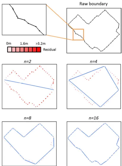
The obtained raw boundaries usually exhibit a zigzag pattern along the derived outlines, as shown in the close-up of Figure 2. To provide a meaningful and compact description of the boundary, polygon simplification is critical to preserve relevant edges. Rather than using the original DP algorithm for polygon approximation (Jwa et al., 2008; Kim and Shan, 2011; Weidner and Förstner, 1995), a Vertex-driven Douglas-Peucker (VDP) algorithm is proposed to simplify a polygon from its raw boundary. The main difference between the two algorithms is that VDP focuses on polygonal complexity while the original DP considers data deviation. In VDP the number of key points, denoted as , is required to generate a polygonal hypothesis, and the optimal value of n is determined through energy minimization in the sequential optimal polygon selection process. This is in contrast to the original DP algorithm relying on a pre-defined point-to-edge distance which is difficult to optimize. Obviously, when the number of the key points is defined as two, the polygonal approximation will appear as a line segment which mutual links the farthest data points to minimize data distortion. With increasing, the polygon expands by iteratively adding the point with the farthest point-to-edge distance to the current form polygon. Figure 2 shows the shapes of various polygonal hypotheses with different . It is clear that the lower the degree of simplification, the lower the amount of data fitting error, but the higher the complexity of the polygon.
Figure 2. Polygonal hypotheses with different numbers of vertices.
3.3 Optimal Polygon Selection
In order to select the optimal polygon among the different hypotheses, the energy function is adopted to globally present the combination of the cost of overall data and the model. According to the general form of the energy function in Eq. 1, the data energy depends on the capability of describing data using a polygon . Thus, the data energy is defined as the
residual error of each point towards the hypothesis polygon. Since a building footprint can be represented as a simple polygon, the complexity of the polygon can be employed as a model constraint. The complexity of a polygon model can be estimated from the LiDAR points along the building boundary. As the vertices of the polygon are a subset of the boundary points, a sequence of coordinate (X, Y) values encodes the polygonal complexity. To simplify computation, a 2D bounding box enclosing the polygon is employed to indicate coordinate range. In this formulation, the global energy function, denoted as , , is defined as a combination of | , which encodes the energy of data over the polygon , and the energy of itself. The global energy function , can be expressed as
, (2)
where is the sum of the squared residuals, is the number of polygon vertices (defined in VDP) and is the area of the data bounding box, which represents the coordinate range. is introduced to balance data and prior terms. We set 1
which is applicable in most cases.
The best polygon representing the building footprint can be found when the overall energy is minimal. In this paper, we adopted the brute-force searching (BFS) strategy to find minimum energy (Enqvist et al., 2011). In other words, the optimal value of n is derived by iteratively calculating and comparing the energy with in the range of "3, $%, where $ is the number of data points. Taking the boundary in Figure 2 as an example, the data energy term ( | ), the prior energy term ( ) and the combination energy term , of each is shown in Figure 3. | drops swiftly when increasing from 4 to 8 and closes to 0 after 9 while grows linearly with increasing n. From the , , the polygon with
8 has the minimum total energy and thus is the corresponding polygon of the best approximation of the building footprint.
Figure 3. Energies for different vertex numbers
4. HYBRID RECONSTRUCTION
4.1 Explicit Reconstruction
It can be observed that the preliminary boundary is typically irregular because key points are the subset of raw boundary points. Therefore, a regularization step is often necessary to enhance the geometric shape of building footprint, such as parallelism and perpendicularity.
A local adjustment is firstly applied on each edge to approximate the real direction. Let ( )* , * , … , * , be the ISPRS Annals of the Photogrammetry, Remote Sensing and Spatial Information Sciences, Volume II-3, 2014
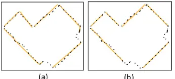
key points of preliminary polygon. The adjusted line -.,-/ is determined by a RANSAC line fitting method using the LiDAR points between * and * . An example is shown in Figure 4(a). Note that angular difference before and after adjustment may represent a dramatic difference for some edges. Therefore, edges with large direction difference from the preliminary polygon (more than 20°), or with small length (less than 2m), are eliminated. Thereafter, this approach explores the direction relationship among line segments. If the angular difference between the potential line and the longest line is close to 0° or 90°, then the regularity relationship is built as parallelism or perpendicularity.
If direction alignment is directly applied to the longest line, the quality of the dominant direction is mainly dependent upon the local fitting of the longest line. Therefore, global adjustment is applied to find the precise dominant direction as well as the optimal parameters for each edge. The data fitting error 0 is used to measure the deviation of points from the fitted line segments, and it is expressed as the accumulation of squared Euclidean distance between each point and the corresponding segment line (Fisher, 2004):
0 ∑:∈;∑ 3∈:234 567, 8 (3)
Here, is one of long line segments < and 67is an observation on . 4 (67, ) represents the squared distance of a point 67 to its corresponding line, which has an associated measurement uncertainty weight 23 (Kanatani, 2008). 23 is set to 1 if the line segment has the direction relationship with the longest line segment and to zero otherwise.
In order to minimize 0 and meanwhile maintain direction relationships, an error minimization optimization approach is employed. As distinct from the energy function defined in Equation 1, where the energy is an accumulation of soft constraints from data and from prior knowledge, the direction relations are considered as equal hard constraints. The objective error function with equal constraints is defined as
=> ( 0 ), ? ∈ @A (4)
where ? is the direction constraint. @A includes parallelism and perpendicularity constraints. The well-known non-linear convex point approach (Vanderbei and Shanno, 1999) is applied to solve the optimization problem. The regularized result of the local fitting of building edges in Figure 4(a) is shown in Figure 4(b). It can be seen that the line segments in Figure 4(b) better represent the shape of the building footprint than those in Figure 4(a).
Figure 4. Explicit reconstruction of building footprint: (a) local fitting and (b) regularization of remaining line segments
4.2 Implicit Reconstruction
As shown in the previous section, short line segments have been eliminated in the explicit reconstruction. The fitted short line
segments usually contain only a few LiDAR points, therefore they are not reliable to represent a building edge, particularly when the density of LiDAR points is not high. The uneven distribution of points due to an irregular scanning pattern makes the situation even worse. Short segments usually link neighbouring long segments. They are referred to as connectors in the following and they will again be reconstructed using energy minimization. However, since robust features cannot be reliably extracted from the limited observations, the connectors will be reconstructed implicitly and a different definition of energy will be necessary. Three types of connector hypotheses are categorized as follows (see also in Figure 5):
a. No additional line: two adjusted line segments are directly connected by a line extension to bridge the gap (Figure 5a).
b. One additional line: use one line to intersect two fixed line segments. The additional line is defined by one observation point and a floating direction (Figure 5b). c. Two additional lines: use two rays to intersect two fixed
line segments. The two rays are defined at one observation point with two floating directions (Figure 5c)
Figure 5. Connector hypotheses: (a) no additional line; (b) one additional line and (c) two additional lines
The optimal connector model is also selected by energy minimization. Unlike the global energy for polygon selection, in Section 3.3, model selection is performed locally on each gap and the data observations are the points between the two adjacent lines. The data energy is defined as the residuals describing the deviation of boundary points from the model. A low residual implies more agreement with the hypothesis model. To describe the prior energy, both shape complexity and smoothness are encoded. Thus, the model energy is extended by adding two more smoothness constraints: (1) length of additional line (favouring short length), and (2) angle transition (preferring right angle). The total energy can be further expressed as
< ( , ) (B CD C ∑ E
∠A B) (5)
where is the area of the bounding box from local observation data; C the extended length of the two line segments; B the number of new added vertices; CD the length of the connector model; E∠A the angle penalty, where E∠A 0 if H 90° J 180° and E∠A 1 otherwise; and the weight coefficient to trade-off between the data term and model term. The result of the connection procedure onto the discretized line segments of Figure 4(b) is shown in Figure 6. It can be seen that the gaps are closed, and the obtained polygon represents well the building footprint. At the bottom-right of the footprint, both smoothness prior and data fitness drive the two additional lines intersecting at the point which is near to the real corner. ISPRS Annals of the Photogrammetry, Remote Sensing and Spatial Information Sciences, Volume II-3, 2014
Figure 6. Watertight building footprint
5. EXPERIMENTS AND DISCUSSION
This section presents the performance evaluation of the developed algorithms for building footprint extraction using energy minimization based explicit and implicit reconstruction. The criteria for quantitative assessment of performance are first introduced. Simulated data with various noise levels was initially used to illustrate the robustness of the developed approach when compared to the DP method for preliminary polygon selection and explicit reconstruction for building footprint extraction. Following this, the results from a real dataset over a large area are presented. The performance was quantitatively evaluated using manually extracted precise reference data.
5.1 Criteria for Quality Assessment
Five evaluation metrics, defined as follows, were used for the quantitative evaluation of performance:
− Coverage Error (CE) evaluates how completely the
approach is able to represent the ground-truth polygon. Coverage percentage is expressed as
@ K L KLK K MK K L LLK K MKNO (6)
where the difference analysis between two polygons is based on the Vatti clipping algorithm (Vatti, 1992), implemented in General Polygon Clipper (GPC) software library (http://www.cs.man.ac.uk/~toby/alan/software)
− Root Mean Square Error (RMSE) predicts the deviation of
the footprint to the data. Let $ be the number of boundary points and be the squared residual accumulated from all boundary points, then the RMSE is defined as
PQC R S (7)
− Direction Difference (DD) measures the difference of the
principal orientation between the extracted polygon and the ground-truth polygon. Given the dominant direction of an estimated polygon 4Tand the corresponding ground-truth dominant direction 4, DD is calculated as
U? V (4TW⋅ 4) (8)
− Model Complexity Difference (MCD) aims to reflect the
complexity difference between the derived footprint and the ground-truth. Let and be the number of vertices of the derived polygon and reference polygon, respectively, then MCD is expressed as
Q@ RX Y Z
Z [ (9)
− Vertex Difference (VD) evaluates the likelihood between
the derived footprint and the ground-truth. Let J be the residual distance of a vertex of the derived polygon to the nearest vertex of the reference polygon, then VD is defined as
\ R ∑ J (10)
5.2 Performance on Simulated Data
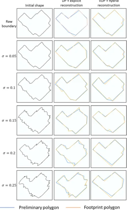
The simulated data were designed to evaluate the developed VDP approach for polygon simplification and extraction of relevant edges from noise influenced boundary points. Gaussian noise with five noise levels (σ 0.05, 0.1, 0.15, 0.2, 0.25m) were added to raw boundary points. Both conventional DP and VDP algorithms were applied. Furthermore, the performance of explicit reconstruction (Sampath and Shan, 2007) with conventional DP and the hybrid reconstruction with VDP presented in this paper were evaluated.
Figure 7. Comparison of performance under various Gaussian noise levels
Figure 7 illustrates the results of DP and VDP for polygonal simplification (blue lines). The results of DP and VDP are quite similar when the noise level is low. However, DP presents an ISPRS Annals of the Photogrammetry, Remote Sensing and Spatial Information Sciences, Volume II-3, 2014
over-fitting of the preliminary boundary when the noise level is high. This is because DP only relies on the local point-to-edge distance to locate the key points. As seen in the DP result with σ 0.25, noisy vertices were not eliminated in the left part of the figure. With the preliminary polygon, explicit reconstruction generates an irregular footprint since the rule based on angle difference does not work well on noisy boundaries. On the other hand, VDP considers the global data deviation as well as model complexity to control the key point selection. A key point is added to the preliminary polygon only when the alleviation of data distortion is larger than the cost of introduction of a new vertex. Consequently, the hybrid reconstruction based on VDP achieves a regular polygon shape. The metric evaluation in Table 1 indicates that the hybrid method has a low direction difference as the dominant direction is measured by global optimization rather than via local adjustment. MCD for both methods increased at a higher level of noise. Explicit reconstruction exhibits an overestimation result, while hybrid reconstruction shows a result of underestimation. However, the model complexity of the hybrid method is closer to the ground truth. In addition, much smaller values of vertex difference achieved from VDP approximation and hybrid reconstruction suggest better performance than the explicit method.
CE RMSE DD MCD VD
σ=0.05m DP 0.01 0.25 0.04 0.18 0.65
VDP 0.02 0.24 0.02 0.00 0.42
σ=0.10m DP 0.03 0.31 0.16 0.18 2.67
VDP 0.04 0.25 0.02 0.00 0.23
σ=0.15m DP 0.08 0.39 0.12 0.09 1.20
VDP 0.09 0.38 0.03 0.09 0.40
σ=0.20m DP 0.12 0.54 0.21 0.45 3.06
VDP 0.11 0.44 0.07 0.18 0.52
σ=0.25m DP 0.16 0.59 0.32 0.73 3.26
VDP 0.14 0.53 0.12 0.27 0.82 Table 1: Statistical assessment under various Gaussian noise levels.
5.3 Performance on Real Data
Experiments have been conducted over the urban area of Eltham, Victoria, Australia. This site, with well vegetated rolling terrain, is located northeast of the Melbourne CBD. The LiDAR data was collected by an Optech Gemini scanner with an average point spacing of ~0.55m. In addition, aerial imagery was available for this site and this was employed as an independent data source in the evaluation.
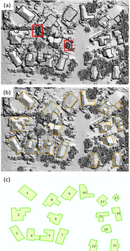
The developed approach was applied to the whole dataset, and the results of a portion containing 17 buildings, whose reference data were available, are presented in Figure 8. The detected building regions shown in Figure 8(a) are indicated by black lines overlaid on the hill-shaded DSM image. The small patches on dense tree crowns, highlighted by red squares, are falsely detected building regions. These are subsequently removed by an area-based filtering algorithm. All 17 building regions were detected. The results of preliminary extracted polygons and the final derived footprints, obtained using the proposed approach, are represented in blue and orange, respectively, in Figure 8(b). The reference footprints were generated by manual delineation with the assistance of aerial photography. These are shown by the green polygons in Figure 8(c).
Table 2 shows assessment result for the reconstruction of the 17 buildings. As indicated in the table, the coverage error is
relatively high when rooftops are occluded by trees (e.g. b11, b16 and b17). Consequently, the vertex difference of these buildings is also relatively high. Another factor contributing to the vertex difference is the model complexity difference. The MCD is caused by either overestimation (e.g. b5 and b9) or underestimation (e.g. b7 and b12). The reconstructed footprints fit the data typically well as the RMSE is small, in the range of 0.18-0.77m. The largest RMSE is from b7 because a small protrusion in the right side is not reconstructed. For direction difference, all reconstruction results show a small deviation to the corresponding reference footprints. The small standard deviations of all evaluation criteria indicate that the proposed method has a reliable and consistent performance.
Figure 8. Building footprint reconstruction: (a) the detected buildings, (b) reconstructed footprints and (c) ground truth.
Building CE RMSE DD MCD VD
b1 0.13 0.21 0.02 0.00 0.29
b2 0.01 0.18 0.01 0.00 0.48
b3 0.14 0.53 0.00 0.00 0.43
b4 0.03 0.53 0.03 0.00 0.38
b5 0.18 0.63 0.02 0.22 1.94
b6 0.10 0.49 0.02 0.00 0.57 b7 0.10 0.77 0.00 0.29 0.77 ISPRS Annals of the Photogrammetry, Remote Sensing and Spatial Information Sciences, Volume II-3, 2014
b8 0.14 0.48 0.03 0.09 0.54 b9 0.18 0.33 0.03 0.14 3.69
b10 0.04 0.38 0.01 0.27 0.79
b11 0.24 0.47 0.06 0.00 1.16
b12 0.11 0.21 0.05 0.00 1.13
b13 0.00 0.35 0.07 0.00 0.54
b14 0.05 0.56 0.09 0.22 0.54
b15 0.01 0.30 0.02 0.00 0.31
b16 0.24 0.38 0.03 0.00 0.51
b17 0.22 0.42 0.01 0.29 0.56
Average 0.11 0.42 0.03 0.09 0.86
Std 0.08 0.15 0.02 0.12 0.81 Table 2: Statistical assessment of building footprint reconstruction.
5.4 Discussion
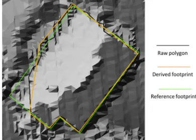
Several factors have an impact on the results of building footprint reconstruction. The point density within LiDAR point clouds and the sensor scanning pattern directly influence the quality of the results. The proposed approach comprises a number of processing steps and each has an impact on the subsequent processes, and thus on the final results. An example is given in Figure 9, which highlights the difference between the boundary of the detected building area, the reconstructed footprint and the ground-truth of b9 (c.f. Figure 8). The error is caused by misclassification of a low-level building component at the lower left corner as ground and this error propagates to the boundary of the building outlines, resulting in incorrect footprint.
Figure 9. Difference between raw boundary and ground truth.
The other challenge is the selection of the proper weight parameters in Eq. 5. In the current implementation, the weights are determined manually, by trial and error comparing with the reference data, and then the constant 0.5 is used for other buildings. However, the value is not always effective and can lead to incorrect generation of short line segments in implicit reconstruction, as shown in b5 and b12 of Figure 8. An adaptive is necessary to determine based on the local environment.
Nonetheless, these errors can be largely avoided through an increase in the point density of the LiDAR data. An example is given in Figure 10 where the point spacing is ~0.23m and the point density around 4 times that of the data shown in Figure 8. It is clear that the building footprints are correctly reconstructed, despite their complex structure and varying size. Even small structures with extremely short boundary segments are accurately reconstructed and modelled.
Figure 10. Footprint reconstruction of complex buildings with high density LiDAR data.
6. CONCLUDING REMARKS
This paper has presented a novel energy minimization based method for building footprint extraction from airborne LiDAR data. A number of component algorithms have been developed. Rather than utilising a pre-defined threshold for polygonal simplification, the vertex-driven Douglas-Peucker method has been proposed to improve performance. Different forms of energy minimization are formulated to determine the optimal polygon among various hypotheses, and to bridge gaps between consecutive line segments through optimal connectors. In summary, the paper has made three principal contributions:
− A combined global energy function encoding data energy and prior energy for determination of the best polygonal simplification, where the model complexity is controlled by the number of vertices obtained from the vertex-driven DP algorithm;
− An explicit reconstruction incorporating geometric knowledge of buildings (parallelism and perpendicularity) in a global optimization to improve robustness and accuracy; and
− An implicit reconstruction through a connector structure to ensure completeness and topological correctness of the building polygon.
The proposed approach has been experimentally tested and evaluated with both simulated and real data over large urban test areas. Quantitative assessment of the resulting building footprints against accurate reference data, using various quality criteria, has shown that the developed approach displays a high level of robustness and reliability. The experiments conducted have also shown that even better performance can be achieved with LiDAR data of a higher point density.
It is noteworthy that the developed approach assumes that building footprints consist of sets of piecewise linear segments. While this is true for the majority of buildings, those with ‘special’ structural characteristics, such as domed and curved structures, are not uncommon. Improvement of the current approach or development of new methods is warranted to accommodate these cases.
ACKNOWLEDGEMENTS
The authors would like to thank the Department of Environment and Primary Industries of Victoria (www.depi.vic.gov.au) for providing the LiDAR data of Eltham. We also appreciate the reviewers’ constructive feedback for improving this paper. ISPRS Annals of the Photogrammetry, Remote Sensing and Spatial Information Sciences, Volume II-3, 2014
REFERENCES
Alharthy, A., Bethel, J., 2002. Heuristic filtering and 3D feature extraction from LiDAR data. Int. Arch. Photogramm. Remote Sens. Spat. Inf. Sci. XXXIV, 23–28.
Arefi, H., Reinartz, P., 2013. Building reconstruction using DSM and orthorectified images. Remote Sens. 5, 1681–1703.
Bernardini, F., Bajaj, C., 1997. Sampling and reconstructing manifolds using alpha-shapes, in: 9th Canadian Conference on Computational Geometry. pp. 193–198.
Boykov, Y., Jolly, M., 2001. Interactive graph cuts for optimal boundary & region segmentation of objects in ND images. Int. Conf. Comput. Vis. 1, 105–112.
Boykov, Y., Veksler, O., Zabih, R., 1999. A new algorithm for energy minimization with discontinuities, in: IEEE International Workshop on Energy Minimization Methods in Computer Vision (EMMCVPR). pp. 205–220.
Dorninger, P., Pfeifer, N., 2008. A comprehensive automated 3D approach for building extraction, reconstruction, and regularization from airborne laser scanning point clouds. Sensors 8, 7323–7343.
Douglas, D., Peucker, T., 1973. Algorithms for the reduction of the number of points required for represent a digitzed line or its caricature. Can. Cartogr. 10, 112–122.
Enqvist, O., Jiang, F., Kahl, F., 2011. A brute-force algorithm for reconstructing a scene from two projections. CVPR’11 2961–2968.
Fisher, R.B., 2004. Applying knowledge to reverse engineering problems. Comput. Des. 36, 501–510.
Geman, S., Geman, D., 1984. Stochastic relaxation, Gibbs distributions, and the Bayesian restoration of images. IEEE Trans. Pattern Anal. Mach. Intell. 6, 721–741.
Huang, H., Sester, M., 2011. A hybrid approach to extraction and refinement of building footprints from airborne LiDAR data. Int. Arch. Photogramm. Remote Sens. Spat. Inf. Sci. XXXVIII, 153–158.
Jwa, Y., Sohn, G., Cho, W., Tao, V., 2008. An implicit geometric regularization of 3D building shape using airborne lidar data. Int. Arch. Photogramm. Remote Sens. Spat. Inf. Sci. XXXVII, 69–75.
Kabolizade, M., Ebadi, H., Ahmadi, S., 2010. An improved snake model for automatic extraction of buildings from urban aerial images and LiDAR data. Comput. Environ. Urban Syst. 34, 435–441.
Kanatani, K., 2008. Statistical optimization for geometric fitting: Theoretical accuracy bound and high order error analysis. Int. J. Comput. Vis. 41, 73–92.
Kim, K., Shan, J., 2011. Building footprints extraction of dense residential areas from LiDAR data local planarity. Annu. Conf. Am. Soc. Photogramm. Remote Sens. WI, 193–198.
Kolmogorov, V., Zabih, R., 2002. Multi-camera scene reconstruction via graph cuts. Eur. Conf. Comput. Vis. 82–96.
Lafarge, F., Descombes, X., Zerubia, J., Pierrot-Deseilligny, M., 2008. Automatic building extraction from DEMs using an object approach and application to the 3D-city modeling. ISPRS J. Photogramm. Remote Sens. 63, 365–381.
Lafarge, F., Mallet, C., 2012. Creating large-scale city models from 3D-point clouds: A robust approach with hybrid representation. Int. J. Comput. Vis. 1, 69–85.
Neidhart, H., Sester, M., 2008. Extraction of building ground plans from LiDAR data. Int. Arch. Photogramm. Remote Sens. Spat. Inf. Sci. XXXVII, 405–410.
Sampath, A., Shan, J., 2007. Building boundary tracing and regularization from airborne LiDAR point clouds. Photogramm. Eng. Remote Sensing 73, 805–812.
Sester, M., Neidhart, H., 2008. Reconstruction of building ground plans from laser scanner data, in: AGILE08. pp. 1–11.
Shapovalov, R., Velizhev, A., Barinova, O., 2010. Non-associative markov networks for 3D point cloud classification. Int. Arch. Photogramm. Remote Sens. Spat. Inf. Sci. XXXVIII, 103–108.
Vanderbei, R., Shanno, D., 1999. An interior-point algorithm for nonconvex nonlinear programming. Comput. Optim. Appl. 13, 1–20.
Vatti, B., 1992. A generic solution to polygon clipping. Commun. ACM 35, 56–63.
Vosselman, G., 1999. Building reconstruction using planar faces in very high density height data. Int. Arch. Photogramm. Remote Sens. Spat. Inf. Sci. XXXII, 87–92.
Vosselman, G., 2002. Fusion of laser scanning data, maps, and aerial photographs for building reconstruction, in: IEEE International Geoscience and Remote Sensing Symposium and the 24th Canadian Symposium on Remote Sensing (IGARSS’02). pp. 85–88.
Wang, H., Daphne, K., 2013. Subproblem-tree calibration: A unified approach to max-product message passing, in: Proceedings of the 30th International Conference on Machine Learning. pp. 190–198.
Wang, O., Lodha, S.K., Helmbold, D.P., 2006. A Bayesian approach to building footprint extraction from aerial LIDAR data, in: Third International Symposium on 3D Data Processing, Visualization, and Transmission (3DPVT’06). pp. 192–199.
Weidner, U., Förstner, W., 1995. Towards automatic building extraction from high-resolution digital elevation models. ISPRS J. Photogramm. Remote Sens. 50, 38–49.
Yang, M.Y., Förstner, W., 2011. Regionwise classification of building facade images. Photogramm. Image Anal. XXXVIII, 209–220.
Zhou, Q.-Y., Neumann, U., 2008. Fast and extensible building modeling from airborne LiDAR data. Proc. 16th ACM SIGSPATIAL Int. Conf. Adv. Geogr. Inf. Syst. (on CD–ROM).
Zhou, Q.-Y., Neumann, U., 2010. 2.5 D dual contouring: a robust approach to creating building models from Aerial LiDAR point clouds. Eur. Conf. Comput. Vis. 115–128.