A LINE-BASED APPROACH FOR PRECISE EXTRACTION OF ROAD AND CURB
REGION FROM MOBILE MAPPING DATA
Ryuji Miyazakia∗
, Makoto Yamamotob, Eiji Hanamotob, Hiroaki Izumiband Koichi Haradac
a
Faculy of Psychological Science, Hiroshima International University, 555-36, Gakuendai, Kurose, Higashi-hiroshima, Hiroshima, Japan.
Sanei Co., 3-26, Kaminobori-cho, Nakaku, Hiroshima-city, Hiroshima, Japan. (makoto, hanamoto, izumi)@sanei.co.jp
cGraduate School of Engineering, Hiroshima University, 1-4-1, Kagamiyama, Higashi-hiroshima, Hiroshima, Japan.
KEY WORDS: MMS, point cloud, planar structure, boundary, uneven distribution density, region growing, curbstone.
ABSTRACT:
Planar structure detection from point clouds is important process in many applications such as maintenance of infrastructure facility including roads and curbs because most artificial structures consists of planar surfaces. The Mobile Mapping System can obtain a large amount of points with traveling at a standard speed. However, in the case that the high-end laser scanning system is equipped, the distribution density of points is uneven. In the point-based method, this situation causes the problem to the method of calculating geometric information using neighborhood points. In this paper, we propose a line-based region growing method in order to detect planar structures with precise boundary from point clouds with uneven distribution density of points. The precise boundary of a planar structure is maintained by appropriately creating line segments from the input clouds. We adapt the definition of neighborhood and the estimation of the normal vector to the line-based region growing. The evaluation by comparing our result with manually extracted points shows that more than 98% of curb points are detected. And, about 90% of the boundary points between a road and a curb are detected with less than 0.005 meters of the distance error.
1 INTRODUCTION
A recent development of three dimensional laser scanning system make it possible to obtain high density point cloud easily. The Mobile Mapping System (MMS) which is equipped with such a high density laser scanning system can measure the environment around a road precisely by simply traveling on the road at a stan-dard speed. Therefore, the traffic regulation is not needed to mea-sure the environments around road by MMS. This is very helpful to the survey of road environment for the purpose of maintenance and management.
An application of a large scale three dimensional point cloud for the management of the infrastructure facilities like road en-vironments is one of the important topics. Numerous techniques are offered to utilize a point cloud for practical purpose (Mertz, 2011),(Aoki et al., 2012). In particular, the planar structure detec-tion from a point cloud is an important technique because artifi-cial facilities are often constituted by planar surfaces. Demantk´e et al. focus on facade in order to utilize point cloud data for sev-eral purposes including localization of autonomous vehicles, reg-istration of point cloud and fine building modeling (Demantk´e et al., 2012), (Demantk´e et al., 2013).
Belton et al. proposed a method for automating some of the pro-cessof road scenes including defining the road and the curbs from unorganized point data(Belton and Bae, 2010). Their method di-vides point cloud into a set of grid. Then, the ground points are extracted by using the linear regression for ordered vertical values of points in each grid. Then, the region growing is applied with respect to the grids in order to merge the ground points. The curb points are also defined by using information of the points in the grid. The curb is considered to exist in the the grid which includes the edge of the road region or is adjacent to the grid including the
∗Corresponding author.
edge of the road. In such a grid, the 2D cross section of points is created and the edge of the curb is detected. The difficulty of this method is in setting of the grid size. The grid size should be large enough to contain significant number of points, but also small enough so that a very small number of salient features be present.
Eigenvalues and eigenvectors of the covariance matrix are often calculated within the local neighborhood area of the query point in order to characterize geometric property at that point. The nor-mal vector at the point is defined as the eigenvector which cor-responds to the largest eigenvalue. El-Halawany et al. proposed the method to detect road curbs from a point cloud by using such an information(El-Halawany et al., 2011). They segment ground point from a point cloud by thresholding eigenvalues and the an-gle of the normal vector to the horizontal plane. Other objects including walls or poles are segmented by changing thresholds.
Bremer et al. also used eigenvalues for object extraction from a point cloud(Bremer et al., 2013). They proposed multi scale fea-ture computation method that uses two sets of eigenvalues com-puted from different size of neighborhood regions.
In such a method, precision of the boundary between segmented regions depends on the size of the neighborhood area. The size of the neighborhood area should be large enough so that the effect of noise is as small as possible. However, the wide neighborhood area causes the disappearance of relatively small changes in the estimation of geometric property. Furthermore, it is difficult to estimate the normal vector around the edge where planar struc-tures are adjacent each other.
On the other hand, other methods which use straight line seg-ments as the basic element are proposed. A line segment is cre-ated from a sequence of points which is arranged in a straight line. These method are based on the idea that the points in each scan line belonging to a surface of a planar structure form a straight line. He et al. proposed the method of detecting planar structures by a line-based spectral clustering from airborne LiDAR data(He et al., 2013). In the case of airborne LiDAR data, the interest pla-nar structure is a roof of a building. It is unclear that there method can apply to the nearly planar surface like a road which is gently curved.
For the purpose of road maintenance, there is the case that re-quires very high precision in some situations. For example, ac-cording to Japan Road Association, the depth of a rut is mea-sured in the precision of millimeters. And, it is considered that a rut should be repaired if the depth exceeds a few centimeters. Re-cent high density laser scanning system can obtain the point cloud which satisfies the demand of such a high precision. Furthermore, structures of road environment including road and curbstone must be extracted in similar accuracy in order to automate the assess-ment for road maintenance. However, it is often difficult to apply existing algorithms to the measured data by the MMS equipped with the high density laser scanning system, due to the character-istics of such a data.
This paper is aimed to precisely detecting the planar structure from a point cloud measured by the MMS with the high-end laser scanning system. In particular, we focus on precise detection of the boundary of planar structures and detecting relatively small planar structure like a curb.
Our approach is the line-based region growing method. In prac-tice, roads often have a roll and there are ruts on a road. More-over, a curb might be bent. So, the surfaces of roads and curbs are not strictly planar although they are locally considered as a pla-nar. The region growing approach is appropriate to detect such a structure. However, the point-based region growing includes a disadvantage to the point cloud which is measured by the MMS equipped with the high-end laser scanner.
We tackle the problem to precise processing of such a data by the line-based approach. Our proposal creates line segments by creating a polyline from a point sequence of which a point cloud is segmented into scan lines. If a point sequence is approximated by a polyline appropriately, vertices of a polyline are assigned to the boundary of structures precisely. Therefore, we use line segments as elements for the region growing in order to precisely detect the boundary of structures.
The planar structure detection by the region growing needs the definition of neighborhood and the estimation of a normal vector. In the point-based approach, the neighborhood of a target point is simply defined using the distance between points. The normal vector at a point is estimated by least squares fitting within neigh-borhood points. However, these cannot be applied to the line-based approach directly. We adapt the definition of the neighbor-hood and the estimation of the normal vector in order to achieve the line-based planar structure detection by region growing in this paper.
The advantage of our proposal over ordinary point-based methods is that the boundary of planar structures is precisely kept. This is because the element for planar structure detection is the line segment which is created so that an end point of a line segment is placed at the boundary. On the other hand, it is difficult to detect boundary points by ordinary point-based methods because the normal vector which defines the direction of a plane surface is estimated from a certain range of neighborhood points.
2 METHOD
2.1 Utilized data
The point cloud which is obtained by MMS with the high density laser scanning system share the characteristics in distribution of points. Recent laser scanning system can measure up to a million points per second. In the direction traversing a road, points are measured very dense. Actually, the interval of measrued points is often a few millimeters.
However, the interval of measured points along the direction of which the MMS travels depends on the rotating speed of the laser irradiation part and the speed of which the MMS travels. The ro-tation period of the laser irradiation part is much longer compared to the laser irradiation period. The measurement interval along the direction the MMS travels is often about a few hundreds of millimeters. So, the density of point distribution is greatly unbal-anced with the direction (Figure 1).
Figure 1: The difference of point density according to the direc-tion.
(a) Enough range to define the neighborhood.
(b) Too narrow range.
Figure 2: The necessity of wide neighborhood range.
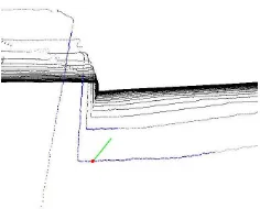
This situation causes the problem to the method of calculating ge-ometric information using neighborhood points because it is nec-essary to define the neighborhood range too wide in the sparse direction (Figure 2(a)). If the neighborhood range is not wide enough, the neighborhood includes points in one direction only (Figure 2(b)). For example, if the range of neighborhood is de-fined too wide in estimating the normal vector, we cannot es-timate it precisely at the point on the planar region around the boundary of structures. Figure 3 shows an example of such a case. The estimated normal vector is tilting because the neigh-borhood region includes points of vertical plane even though the target point is on the horizontal plane.
Figure 3: The estimated normal vector at the point around the boundary. The green line is the normal vector at the point col-ored red. Small blue dots are the neighborhood points used for estimating the normal vector.
(a) The region growing pro-cess stopped in front of the boundary.
(b) The region exceeds the appropriate boundary.
Figure 4: Examples of road detection by the point-based region growing. The detected road points are colored in red.
shows an example of the road detection by a little larger threshold (15 degrees). The region exceeds the boundary between the road and the curb.
2.2 Line segment creation
First, we separate the input point cloud into sequences of points that represent scan lines. Each point of input point cloud contains angle information of which the laser has been irradiated. The angle increases monotonically from 0 (degree) to 360 in the same scan line. Then, the angle becomes 0 at the beginning of the next scan line. In practice, there is the case that the 0 degree point is not measured. So, let the beginning of the scan line be the point at which the value of angle decreases from the previous point.
Next, we create a polyline which approximates a sequence of points of each scan line. We use the line segment merging ap-proach for the polyline creation. The process of the polyline cre-ation is as follows. The points in the sequence are ordered by the value of the angle. Let the sequence ofnpoints{p0, p1,· · ·, pn−1} beP S(0,n−1). The initial polyline is created by connecting the pointpiand next pointpi+1, (0≤i≤n−2). Then, we define the approximation errorE(i,j)that the sequence of pointsP S(i,j) is approximated by the line segmentpipjas the equation (1).
E(i,j)= max
pk∈P S(i,j)
(dist(pk, pipj)), (1)
where,dist(pk, pipj)is the perpendicular distance from the point
pkto the line segmentpipj.
The initial polyline is simplified by merging adjacent two line segments. In the simplification process, we select the pair of line segments of which the approximation error after merging is the minimum. The polyline simplification is performed by repeat-ing the segment mergrepeat-ing process until the approximation error exceeds the threshold.
Finally, we obtain polylines of the number of scan lines by apply-ing polyline creation to each scan line. Then we use line segments which constitute polylines as a proxy of a subsequence of points that is approximated by the line segment (Figure 5).
2.3 Line-based region growing
We apply the region growing approach to a set of line segments in order to detect a nearly planar region. In general, the region grow-ing approach starts from selectgrow-ing a seed as the first query. The query is added to the region and the neighborhoods of the query are examined whether should be added to the region. The neigh-borhood which is added to the region becomes the next query in order to grow the region.
In the case of the planar structure detection by the point-based re-gion growing, a data structure like a k-d tree is used for defining neighborhood points. However, another technique is necessary to define the neighborhoods in the line-based case. Zhang et al proposed the method using the cylindrical region whose axis is the query line segment(Zhang and Faugeras, 1992). He et al. also adopted this method to define neighboring line segments(He et al., 2013). Zhang’s method seems to be reasonable for neighbor-hoods detection. But, we have to check all line segments in the previous and the next scan lines.
We use the 3D segment tree(de Berg et al., 1997) for defining neighboring line segments. The 3D segment tree can determine the relation of inclusion and the relation of partially overlap be-tween the intervals in three dimensional space. So, we create ap-propriately three dimensional intervals from line segments, and define neighborhoods of a line segment by the intervals. We use the axis aligned bounding box (AABB) of a line segment for representing the interval of the 3D segment tree. However, if a line segment is aligned parallel to an axis, its AABB is degener-ated. To avoid this situation, The redundancy along each axis is added to a line segment. For the end pointspi= (xi, yi, zi)and
pj = (xj, yj, zj)of a line segmentpipj, letxmin,ymin,zmin,
xmax,ymaxandzmaxbemin(xi, xj),min(yi, yj),min(zi, zj), max(xi, xj), max(yi, yj)andmax(zi, zj), respectively. And,
we define the AABB whose diagonal is the line segment(xmin−
c, ymin−c, zmin−c) (xmax+c, ymax+czmax+c). This AABB
is used for the interval of the 3D segment tree (Figure 6).
Figure 6: Definition of the AABB of a line segment.
The line segment is defined as the neighborhood of the query segment if the line segment satisfies the following two conditions:
Figure 5: An example of the polyline approximating the scan line. Polylines are colored red. Large blue points are vertices of polylines. Original measured points are black dots.
2. The line segment is in the next scan line or the previous scan line of the scan line of the query segment.
An example of defining neighborhood line segment is shown in figure 7. The red line segment is the query line segment and its AABB is drawn in red. The AABB of green line segment par-tially overlaps the AABB of the query line segment. Then, it is defined as the neighborhood line segment of the query line seg-ment. But, the blue line segment whose AABB does not intersect to the AABB of the query line segment is not included in the neighborhoods.
Figure 7: Definition of neighboring line segment.
In the planar structure detection by the region growing, the dif-ference of the angles of the normal vectors is used for examining whether the neighboring primitive is added to the region. The least squares fitting within neighborhoods is often used for es-timating the normal vector. However, the area of the neighbor-hoods will be too wide to precisely estimate the normal vector in the situation mentioned in the section 2.1. So, we adopt the local best-fit plane of the neighborhood line segments for estimating the normal vector at the line segment. The local best-fit plane is defined as the plane which passes the query line segment and includes the neighborhood line segments most. We use the mod-ified version of the local best-fit plane used in (He et al., 2013) in this paper.
Let the query line segment and its neighborhoods beliandN(li),
respectively. The candidate planePi,jis generated from two end
points ofliand the mid-point oflj ∈ N(li). The line segment
lkis defined as an inlier ofPi,jif the distance between thePi,j
and at least one end point oflkis smaller than a threshold and
ni,j·dkis closed to zero, whereni,jis the normal vector ofPi,j
anddkis the direction oflk. We calculate the degree of fit as
the summation of the lengths of the inlier line segments. Then, the candidate plane with the largest degree of fit is defined as the best-fit planePiofli. And, the normal vectorniofPiis used for
the normal vector ofliin the region growing procedure. Figure
8(a) shows an example of the neighborhood line segments. And, Figure 8 shows inliers of the best-fit plane. The line segments colored in cyan are selected as the inliers of the best-fit plane from the neighborhood line segments.
(a) The neighborhood line segments.
(b) The inlier line segments.
Figure 8: An example of inlier line segments of the best-fit plane. The query line segment is colored in red. The green line segments and the cyan line segments are the neighborhoods and the inliers, respectively.
The seed segment is selected by using the degree of fit mentioned above. A large degree of fit means that the target line segment is placed on the large planar region. So, we select the seed segment of the largest degree of fit from line segments that are not assigned to any planar structure yet.
3 EXPERIMENTAL RESULTS
Figure 9: The input point cloud.
Figure 10: The result of creating line segments from the input cloud.
direction traversing a road is a few millimeters. On the other hand, measurement interval along the direction the MMS travels is about 280 millimeters when the MMS runs at 50 kilometers per hour. Figure 9 shows the input point cloud used by this experi-ment. This point cloud consists of one and a half million points.
Figure 10 shows the result of creating line segments from the input cloud. These line segments are created by approximating a point sequence of each scan line. The approximation error is within 0.015 meters. In practical application of planar structure detection, short line segments can be eliminated from target line segments. Intuitively, short line segments tend to be placed on vegetation or small object which belong to irrelevant features. In this experiment, we filter out short line segments whose length is less than 0.05 meters.
Then, the planar structures are detected by our proposal. In this experiment, we use 15 degrees and 0.05 meters as the threshold of the difference of angle of normal vectors and the distance error, respectively.
Figure 11 shows the result of extracting line segments that con-stitue planar structures. In the input point cloud of this experi-ment, there are four planar structures that represent curb regions. We can see that all four curbs are extracted by visual evaluation.
Figure 12 shows the illustration which is focused on the end of a curb. The end of a curb may become lower gradually. It can be seen that such a small planar structure is also detected.
3.1 Evaluation of precision of roads and curbs segmentation
For evaluating the precision of planar structure detection, we fo-cus on roads and curbs. An expert extracts points of curbs man-ually in order to compare with points of curbs extracted by our proposal. Figure 13 shows extracted points for comparison.
Figure 11: The result of detecting planar structures by line-based region growing.
Figure 12: The part of a curb in the result of planar structure detection.
the MMS travels is defined as the point whose angle information shows just under the MMS. Then, we define the ground region according to following two conditions:
• The difference of the angle between the vertical vector and the normal vector of the least squares fitting plane is within 15 degrees.
• All differences of the height between the point under the MMS and line segments in the detected region are within 0.5 meters.
The curb region is discriminated by the following two observa-tions. The curb region is nearly vertical. And, there are ground regions above and under the curb regions. So, the curb region is defined as follows:
• The angle between the vertical vector and the normal vector of the least squares fitting plane is nearly perpendicular. The threshold is 15 degrees in this case.
• More than half of line segments include the ground segment within the neighborhood of both end points.
Figure 13: Manually extracted curb points for comparison.
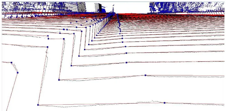
Figure 14: Discrimination of the curb and the ground region.
Figure 14 shows the result of discrimination. The ground region and the curb region are colored in blue and red, respectively.
Discrimination of curbs and roads in this experiment depends on the observation of the input cloud. The environment of curbs and roads will be different in some cases. Robust discrimination such a structure is the future work.
Figure 15: The comparison of extracted curb points. The correct point, the false positive point and the false negative point are colored in green, blue and red, respectively.
Figure 16: An example of manually extracted boundary points (red) and boundary points by our proposal (blue). Magenta color means that the position of both boundary point is match.
not extracted (false negative). An example of the evaluation result is illustrated in Figure 15.
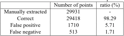
The statistical evaluation of extracted points is tabulated in Table 1. More than 98 % of curb points are extracted by our proposal. And, the missing rate is 1.71 %. Most points of relatively small planar structures like a curb can be extracted by our proposal.
Table 1: The statistical evaluation of extracted points Number of points ratio (%)
Manually extracted 29931
-Correct 29418 98.29
False positive 1710 5.71
False negative 513 1.71
Secondly, we evaluate the precision of detection of the boundary between a curb and a road by the distance error. The boundary points between a curb and a road are also extracted by a expert. And, we regard the point with lower height of a line segment representing a curb as the boundary between a curb and a road.
An example of manually extracted boundary points and boundary points extracted by our proposal is shown in Figure 16. Usually, there are two boundary points in a scan line. One is the left side of a point of which MMS travels. And, the other is on the opposite side. We associate the manually extracted boundary point with the boundary point extracted by our proposal.
Then, the distance error between corresponding points is evalu-ated. In this evaluation, 234 points are manually extracted for comparison. The statistical evaluation of the boundary points ex-traction is tabulated in Tables 2 and 3. Average of the distance error is 0.004 meters and median of the distance error is 0.0022 meters. From Table 3, about 90 percent of boundary points were detected with the precision of 0.005 meters by our proposal.
Figure 17: A part where the distance error is large.
Table 2: The statistical evaluation of the boundary points extrac-tion.
Table 3: The distribution of the distance error. Distance error
(meters) Counts Rate (%) Cumulative rate (%)
∼0.001 58 24.79 24.79
0.001∼0.002 42 17.95 42.74
0.002∼0.003 85 36.32 79.06
0.003∼0.004 9 3.85 82.91
0.004∼0.005 18 7.69 90.60
0.005∼ 22 9.40 100.00
4 CONCLUSIONS AND FUTURE WORK
We presented the method for planar structure detection with pre-cise boundary from a point cloud which has uneven distribution density of points. In the case that points measured by the MMS which is traveling at standard speed, the distribution density of points changes with the direction. The unevenness of point den-sity can be avoided by slowing down the travel of the MMS. However, the utilization of the MMS at a standard speed is the advantage of the MMS. In such a condition of point clouds, a point-based approach has the problem that the neighborhood area has to be set too wide. A line-based approach can keep the pre-cise boundary of structures by creating line segments appropri-ately approximating input points. We created line segments by creating a polyline approximating a sequence of points of each scan line. Moreover, we adopted the 3D segment tree and the best-fit plane in order to adapt the definition of the neighborhood and the estimation of the normal vector for the line-based region growing.
The proposed method was evaluated by comparing with manually extracted curb points. More than 98 % of curb points are correctly extracted by our proposal. Furthermore, about 90% of the bound-ary points between a curb and a road are detected with less than 0.005 meters of the distance error. The distance error at the lo-cation where the surface is deteriorated tends to be large. But,
the boundary points of structures without breakage have been de-tected precisely. In this paper, we evaluated the curb points only. But, other planar structures will be also detected as well.
Automatic reconstruction of three-dimensional models including buildings, roads and curbs is one of the future works. Further-more, we aim to utilize reconstructed models for the management of the infrastructure facilities.
REFERENCES
Aoki, K., Yamamoto, K. and Shimamura, H., 2012. Evalua-tion model for pavement surface distress on 3d point clouds from mobile mapping system. In: International Archives of the Pho-togrammetry, Remote Sensing and Spatial Information Sciences, Vol. XXXIX-B1, pp. 87–90.
Belton, D. and Bae, K.-H., 2010. Automating post-processing of terrestrial laser scanning point clouds for road feature surveys. In: International Archives of Photogrammetry, Remote Sensing and Spatial Information Sciences, Vol. XXXVIII, Part 5, Commission V Symposium, pp. 74–79.
Bremer, M., Wichmann, V. and Rutzinger, M., 2013. Eigenvalue and graph-based object extraction from mobile laser scanning point clouds. In: ISPRS Annals of the Photogrammetry, Remote Sensing and Spatial Information Sciences, Vol. II-5/W2, pp. 55– 60.
de Berg, M., van Kreveld, M., Overmars, M. and Schwarzkopf, O., 1997. Computational Geometry: Algorithms and Applica-tions. Springer-Verlag, Berlin.
Demantk´e, J., Vallet, B. and Paparoditis, N., 2012. Streamed vertical rectangle detection in terrestrial laser scans for facade database production. In: ISPRS Annals of the Photogramme-try, Remote Sensing and Spatial Information Sciences, Vol. I-3, pp. 99–104.
Demantk´e, J., Vallet, B. and Paparoditis, N., 2013. Facade recon-struction with generalized 2.5d grids. In: ISPRS Annals of the Photogrammetry, Remote Sensing and Spatial Information Sci-ences, Vol. II-5/W2, pp. 67–72.
El-Halawany, S., Moussa, A., Lichti, D. D. and El-Sehimy, N., 2011. Detection of road curb from mobile terrestrial laser scan-ner point cloud. In: International Archives of the Photogram-metry, Remote Sensing and Spatial Information Sciences, Vol. XXXVIII-5/W12, pp. 109–114.
He, Y., Zhang, C. and Fraser, C. S., 2013. A line-based spectral clustering method for efficient planar structure extraction from lidar data. In: ISPRS Annals of the Photogrammetry, Remote Sensing and Spatial Information Sciences, Vol. II-5/W2, pp. 103– 108.
Ibrahim, S. and Lichti, D., 2012. Curb-based street floor extrac-tion from mobile terrestrial lidar point cloud. In: Internaextrac-tional Archives of the Photogrammetry, Remote Sensing and Spatial In-formation Sciences, Vol. XXXIX-B5, pp. 193–198.
Mertz, C., 2011. Continuous road damage detection using regular service vehicles. In: Proceedings of the ITS World Congress.