Three dimensional supersonic ow analysis over a satellite
vehicle launcher
A.L. De Bortoli
Federal University of Rio Grande do Sul, Department of Pure and Applied Mathematics, 90501-900, Porto Alegre (RS), Brazil
Received 3 February 1998
Abstract
The ever-widening applications of numerical calculations leads to a variety of new numerical methods, which are dierent in their solution algorithms as well as in the discretization of the governing equations. Despite this development, much work still remains in their improvement towards a fast, accurate and stable convergence. This work shows a numerical method for the solution of compressible and almost incompressible uid ows using a nite volume, explicit Runge-Kutta multistage scheme, with central spatial discretization in combination with multigrid and preconditioning. Numerical tests are carried out for a vehicle launcher for Mach-number 3.75 and 2.0 using the Euler equations. c1999 Elsevier Science B.V. All rights reserved.
Keywords:Supersonic ow; Satellite launcher; Numerical uid ow; Finite volume; Multigrid
1. Introduction
The rapid evolution of computational uid dynamics has been driven by the need of faster and more accurate methods for the calculation of ow elds around congurations of technical interest. With the advent of more powerful computers and more ecient algorithms the researchers have in recent years computed more detailed and sophisticated simulations of uid ow phenomena.
Numerical ow simulations have found their way into the aerodynamical design cycles of aerospace vehicles. Not only do these simulations reduce turn-around time and cost, but they also oer ow parameter variations which are not possible with wind tunnel testing. Even then, ows over aerody-namical congurations display ow phenomena with very dierent scales and with highly nonlinear behaviour.
The design of an aircraft or a launch vehicle involves the calculation of the ow behaviour during a full ight passing through various ow regimes. For transonic and supersonic ows, for example, sharp changes in the aerodynamical coecients are observed due to instabilities presented in the ow. These instabilities are originated not only by strong viscous interactions in the boundary layer,
but also by interactions between the shock wave and boundary layer. This indicates that a model employing the potential ow equations can not be used and one has to employ the Euler/Navier– Stokes equations.
Common methods used for the solution of uid ows are based on nite dierences, nite vol-umes, nite elements and boundary elements discretizations. Each of these methods has its advantages and disadvantages. Nevertheless, all these methods used for the simulation of uid ows have the common feature that the domain has to be divided into a number of small cells of appropriate shape. The solution of the global system of governing equations delivers the variables at the mesh points.
The standard compressible method is employed in this work and consists of the use of the momen-tum equations to obtain the velocity components, the energy equation for the calculation of energy, the mass conservation equation for the computation of density and the state equation to obtain the pressure. The solver employs structured boundary tted meshes with trapezoidal cell shapes.
For all the computations, the Euler/Navier–Stokes equations are solved using the nite vol-ume explicit Runge–Kutta multistage scheme, which can be easily combined with multigrid and preconditioning. Attention is focused on the two major parts of the numerical algorithm. These are the spatial discretization and the time-stepping algorithm. With the spatial discretization of the governing equations we seek to obtain accurate solutions with as few as possible discrete points in the ow domain. Care must be taken to resolve the relevant ow phenomena, i.e., smoothly varying regions of inviscid ows, ow discontinuities as shocks and slip lines. More-over, numerical analysis and well-known experience show that the choice of the spatial discretiza-tion also inuences the convergence of the overall method to the desired steady-state ow regime.
Numerical tests are carried out for a launch vehicle for Mach-numbers 3.75 and 2.0 using the Euler equations. Results obtained for Mach 3.75 are compared with evailable experimental data.
2. Governing equations
The governing equations for nonviscous ows are the Euler equations. The three dimensional Euler equations for unsteady compressible inviscid ows in dierential form reads [6]
and F1, F2 and F3 are the cartesian ux vector components. The total energy and total enthalpy are
E=e+ 12(u2+v2+w2); (3)
H =E+p
; (4)
where q is the velocity vector and e the internal energy. To close this system of equations, the state equation for a perfect gas is employed [7]
p=RT = (−1)[E−1 2(u
2+v2+w2)]; (5)
where R is the gas constant, the specic heat ratio, the uid density, u; vand w are the velocity components, p is the pressure and T the temperature. Eq. (1) can be cast into the integral form [6]
Z
where V and S represent the domain volume and its surface, respectively, and n is the normal vector to the surface.
3. Description of the numerical method
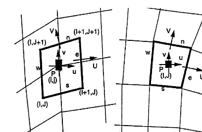
One of the dierences among the various nite volume formulations known in the literature is the arrangement of the control volume for the ow variables [7]. The most frequently used schemes are the cell-centered, cell-vertex and node-centered approachs. Each of these schemes has its advantages and disadvantages. The discretization employed in this work is based on the cell-centered [4], and node-centered arrangements [7], as shown in Fig. 1. As Eq. (1) is valid for an arbitrary control volume, it is also valid for Vi; j; k, which means
The nite volume discretization based on the central averaging is not dissipative [6]. The numerical procedure does not converge to the steady state solution when the high frequency oscillations of error in the solution are not damped. The dissipation vectorDi; j; k is introduced by adding dissipative
uxes as follows [5]:
The dissipation operator is a blend of second and fourth order dierences, and is dened according to [9]
Fig. 1. Node-centered (left) and cell-centered arrangements.
whose dissipation coecient is given by
di+1=2; j; k =i+1=2; j; k[
(2)
i+1=2; j; kxWi; j; k−
(4)
i+1=2; j; kxxxWi−1; j; k]: (10)
The dissipation ux di+1=2; j; k is of third order in smooth regions. However, in regions of high
pressure variations, the dissipation is of rst order and the scheme behaves as a rst order upwind scheme. The dierence operators of rst and third order are x and xxx, respectively,
xWi; j =Wi+1; j−Wi; j; (11)
xxxWi; j =Wi+2; j−3Wi+1; j+ 3Wi; j−Wi−1; j; (12)
and is the scaling factor, which is written for the i direction according to (Blazek, 1994)
i+1=2; j; k = 12(i ∗ i; j; k +
i∗
i+1; j; k); (13)
where the eigenvalues are scaled in each coordinate direction as
ii; j; k∗ =ii; j; k:ii; j; k; (14)
considering the cell aspect ratio
i
The coecients adapted to the local pressure gradients(2) and4), needed to obtain the dissipation
coecient, are written as follows:
(2)i+1=2; j; k =k(2)max(max); (16)
(4)i+1=2; j; k = max(0; k(4)
i; j; k =
pi+1; j; k−2pi; j; k+pi−1; j; k pi+1; j; k+ 2pi; j; k+pi−1; j; k
; (18)
max= (i+2; j; k; i+1; j; k; i; j; k; i−1; j; k); (19)
is the 2nd order divided dierence pressure sensor and k(2) and k(4) are
0:56k(2)60:6; (20)
1 1286k
(4)61
48: (21)
The spectral radius used to control the amount of articial dissipation is dened based on the Mach number M for the i direction according to [2]
i= 1
It is well known that for a central dierence scheme, zero articial viscosity creates numerical diculties. Therefore 2 is chosen according to
2 = max(4M2; ); (23)
where is adopted as [3]
0:1660:6: (24)
4. Time-stepping
In order to obtain numerical solutions of high accuracy, the Runge–Kutta method is chosen [5]. This method is characterized by its low operation count. More than two stages are employed in order to extend the stability region. The following multistage scheme, which requires low computational storage is employed [6]
of convergence of the computed solution. Numerical conditions imposed at the outer boundary should assure that the outgoing waves are not reected back into the ow eld, specially when solving subsonic or mixed ows (regions).
In order to establish an ecient numerical implementation of the boundary conditions the compu-tational domain is surrounded by dummy cells. Using a body tted coordinate system the boundary coinciding with a coordinate line is approximated by a straight lines in the nite volume approxi-mation. On a solid boundary the physical condition of no normal ow can be imposed.
6. Numerical results
In the following, numerical results for a launch vehicle are presented and compared with available data. First computations were performed for launch vehicle for supersonic Mach 3.75. Supersonic ows are high speed ows that appear for reentry launch vehicles or high speed aircrafts. These ows are characterized by strong shocks, contact discontinuities and regions of highly expanded ows.
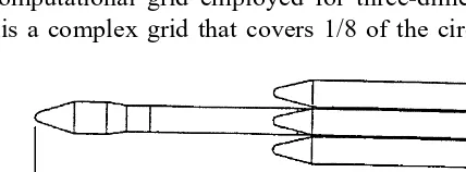
Computations were performed for typical(old) launch vehicle geometry, as shown in Fig. 2. Fig. 3 displays the bidimensional grid for SVL (Satellite Vehicle Launcher) nose, which consists of 62×26 cells. The corresponding pressure coecient is presented in Fig. 4 and is compared with
experimental data [8].
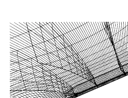
Fig. 5 displays the computational grid employed for three-dimensional geometry, which consists of 140×28×7 cells. It is a complex grid that covers 1/8 of the circumference of the SVL geometry.
Fig. 2. A SVL (Satellite Vehicle Launcher) geometry.
Fig. 4. Comparison of pressure coecient for SVL nose, Mach = 3.75.
Fig. 5. Grid for SVL, 140×26×7 cells.
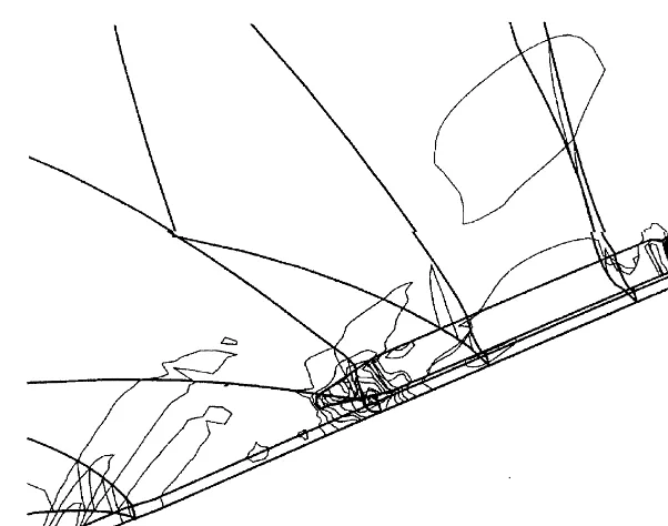
A complete vehicle is obtained reproducing and rotating conveniently this grid. Pressure contours, as presented in Fig. 6, indicate the need for grid renement among the boosters and between the booster and the central body.
Fig. 6. Pressure contours for SVL, Mach = 2.0.
Fig. 7. Color pressure map for 3D launch vehicle, Mach = 2.0.
7. Conclusions
Special care has been taken in the treatment of the inuence of limit coecients used to evaluate the time-step and the articial dissipation. Numerical tests indicate that the dissipation coecient can be chosen between 1/48 and 1/128 without modifying the results.
It is the author’s opinion that the comparison between the experimental and numerical solutions is encouraging. However, a lot of work must still be done in order to obtain and compare the pressure coecient for the complete vehicle geometry.
Acknowledgements
The author would like to thank Dr. Norbert Kroll and Dr. Jiri Blazek for sharing their experi-ences concerning the Euler version of CEVCATS and their many insights into Computational Fluid Dynamics, when he visited DLR – Institute of Design Aerodynamics in Braunschweig (Germany).
References
[1] J. Blazek, Verfahren zur Beschleunigung der Losung der Euler- und Navier–Stokes Gleichungen bei Stationaren Uber-und Hyperschallstromungen, Ph.D. Thesis, University of Braunschweig, 1994.
[2] Y.H. Choi, C.L. Merkle, The application of preconditioning in viscous ows, J. Comput. Phys. 105, (1993) 207–223. [3] A.L. De Bortoli, Solution of incompressible ows using compressible ow solvers, DLR IB 129/94-18, Braunschweig,
Germany, 1994, pp. 1–86.
[4] A.L. De Bortoli, Convergence acceleration applied to solve compressible and incompressible uid ows, J. Brazilian Soc. Mech. Sci., XIX, (3), (1997) 357–370.
[5] A. Jameson, W. Schmidt, E. Turkel, Numerical solution of the Euler equations by nite volume methods using Runge–Kutta time-stepping schemes, AIAA Paper 1981, 81–1259.
[6] N. Kroll, R.K. Jain, Solution of two-dimensional Euler equations – experience with a nite volume code, Forschungsbericht, DFVLR-FB 87-41, Braunschweig, Germany. 1987.
[7] N. Kroll, C.-C. Rossow, Foundations of numerical methods for the solution of Euler equations, Prepared for Lecture F 6.03 of CCG, Braunschweig, Germany, 1989.
[8] C.R. Maliska, A.F.C. Silva, Technical Reports to IAE/CTA – Parts I–IX (1987–1991), Essai du Lanceur Brasilien AU 1/15, December 1988.