ALGORITHMS
ROBERT SEDGEWICK
BROWN UNNER!MY
ADDISON-WESLEY PUBLISHING COMPANY Reading, Massachusetts l Menlo Park, California
To Adam, Brett, Robbie
and especially Linda
This book is in the
Addison-Wesley Series in Computer Science
Consulting Editor Michael A. Harrison
Sponsoring Editor James T. DeWolfe
Library of Congress Cataloging in Publication Data Sedgewick, Robert,
1946-Algorithms.
1. Algorithms. I. Title. QA76.6.S435 1 9 8 3 ISBN O-201 -06672-6
519.4 82-11672
Reproduced by Addison-Wesley from camera-ready copy supplied by the author.
Reprinted with corrections, August 1984
Copyright 0 1983 by Addison-Wesley Publishing Company, Inc.
All rights reserved. No part of this publication may be reproduced, stored in a retrieval system, or transmitted, in any form or by any means, electronic, mechanical, photocopying, recording, or otherwise, without prior written per-mission of the publisher. Printed in the United States of America.
Preface
This book is intended to survey the most important algorithms in use on computers today and to teach fundamental techniques to the growing number of people who are interested in becoming serious computer users. It is ap-propriate for use as a textbook for a second, third or fourth course in computer science: after students have acquired some programming skills and familiarity with computer systems, but before they have specialized courses in advanced areas of computer science or computer applications. Additionally, the book may be useful as a reference for those who already have some familiarity with the material, since it contains a number of computer implementations of useful algorithms.
The book consists of forty chapters which are grouped into seven major parts: mathematical algorithms, sorting, searching, string processing, geomet-ric algorithms, graph algorithms and advanced topics. A major goal in the development of this book has been to bring together the fundamental methods from these diverse areas, in order to provide access to the best methods that we know for solving problems by computer for as many people as pos-sible. The treatment of sorting, searching and string processing (which may not be covered in other courses) is somewhat more complete than the treat-ment of mathematical algorithms (which may be covered in more depth in applied mathematics or engineering courses), or geometric and graph algo-rithms (which may be covered in more depth in advanced computer science courses). Some of the chapters involve mtroductory treatment of advanced material. It is hoped that the descriptions here can provide students with some understanding of the basic properties of fundamental algorithms such as the FFT or the simplex method, while at the same time preparing them to better appreciate the methods when they learn them in advanced courses. The orientation of the book is towards algorithms that are likely to be of practical use. The emphasis is on t,eaching students the tools of their trade to the point that they can confidently implement, run and debug useful algorithms. Full implementations of the methods discussed (in an actual programming language) are included in the text, along with descriptions of the operations of these programs on a consistent set of examples. Though not emphasized, connections to theoretical computer science and the analysis of algorithms are not ignored. When appropriate, analytic results are discussed to illustrate why certain algorithms are preferred. When interesting, the relationship of the practical algorithms being discussed to purely theoretical results is described. More information of the orientation and coverage of the material in the book may be found in the Introduction which follows.
One or two previous courses in computer science are recommended for students to be able to appreciate the material in this book: one course in
. . .
iv
programming in a high-level language such as Pascal, and perhaps another course which teaches fundamental concepts of programming systems. In short, students should be conversant with a modern programming language and have a comfortable understanding of the basic features of modern computer systems. There is some mathematical material which requires knowledge of calculus, but this is isolated within a few chapters and could be skipped.
There is a great deal of flexibility in the way that the material in the book can be taught. To a large extent, the individual chapters in the book can each be read independently of the others. The material can be adapted for use for various courses by selecting perhaps thirty of the forty chapters. An elementary course on “data structures and algorithms” might omit some
of the mathematical algorithms and some of the advanced graph algorithms and other advanced topics, then emphasize the ways in which various data structures are used in the implementation. An intermediate course on “design and analysis of algorithms” might omit some of the more practically-oriented sections, then emphasize the identification and study of the ways in which good algorithms achieve good asymptotic performance. A course on “software tools” might omit the mathematical and advanced algorithmic material, then emphasize means by which the implementations given here can be integrated for use into large programs or systems. Some supplementary material might be required for each of these examples to reflect their particular orientation (on elementary data structures for “data structures and algorithms,” on math-ematical analysis for “design and analysis of algorithms,” and on software engineering techniques for “software tools”); in this book, the emphasis is on the algorithms themselves.
At Brown University, we’ve used preliminary versions of this book in our third course in computer science, which is prerequisite to all later courses. Typically, about one-hundred students take the course, perhaps half of whom are majors. Our experience has been that the breadth of coverage of material in this book provides an “introduction to computer science” for our majors which can later be expanded upon in later courses on analysis of algorithms, systems programming and theoretical computer science, while at the same time providing all the students with a large set of techniques that they can immediately put to good use.
The programs are not intended to be read by themselves, but as part of the surrounding text. This style was chosen as an alternative, for example, to having inline comments. Consistency in style is used whenever possible, so that programs which are similar, look similar. There are 400 exercises, ten following each chapter, which generally divide into one of two types. Most of the exercises are intended to test students’ understanding of material in the text, and ask students to work through an example or apply concepts described in the text. A few of the exercises at the end of each chapter involve implementing and putting together some of the algorithms, perhaps running empirical studies to learn their properties.
Acknowledgments
Many people, too numerous to mention here, have provided me with helpful feedback on earlier drafts of this book. In particular, students and teaching assistants at Brown have suffered through preliminary versions of the material in this book over the past three years. Thanks are due to Trina Avery, Tom Freeman and Janet Incerpi, all of whom carefully read the last two drafts of the book. Janet provided extensive detailed comments and suggestions which helped me fix innumerable technical errors and omissions; Tom ran and checked the programs; and Trina’s copy editing helped me make the text clearer and more nearly correct.
Much of what I’ve written in this book I’ve learned from the teaching and writings of Don Knuth, my thesis advisor at Stanford. Though Don had no
direct influence at all on this work, his presence may be felt in the book, for it was he who put the study of algorithms on a scientific footing that makes a work such as this possible.
Special thanks are due to Janet Incerpi who initially converted the book into QX format, added the thousands of changes I made after the “last draft,” guided the files through various systems to produce printed pages and even wrote the scan conversion routine for Ylj$ that we used to produce draft manuscripts, among many other things.
The text for the book was typeset at the American Mathematical Society; the drawings were done with pen-and-ink by Linda Sedgewick; and the final assembly and printing were done by Addison-Wesley under the guidance of Jim DeWolf. The help of all the people involved is gratefully acknowledged.
Finally, I am very thankful for the support of Brown University and INRIA where I did most of the work on the book, and the Institute for Defense Analyses and the Xerox Palo Alto Research Center, where I did some work
on the book while visiting.
Contents
Introduction . . . . Algorithms, Outline of Topics
1. Preview. . . . Pascal, Euclid’ s Algorithm, Recursion, Analysis of Algorithms
Implementing Algorithms
MATHEMATICAL ALGORITHMS
2. Arithmetic . . . . Polynomials, Matrices, Data Structures
3. Random Numbers . . . . Applications, Linear Congruential Method, Additive
Congruential Method, Testing Randomness, Implementation Notes 4. Polynomials . . . .
Evaluation, Interpolation, Multiplication, Divide-and-conquer Recurrences, Matriz Multiplication
5. Gaussian Elimination . . . . A Simple Example, Outline of the Method, Variations and Extensions 6. Curve Fitting . . . .
Polynomaal Interpolation, Spline Interpolation, Method of Least Squares 7. Integration . . . .
Symbolac Integration, Simple Quadrature Methods, Compound Methods, Adaptive Quadrature
SORTING
8. Elementary Sorting Methods . . . . Rules of the Game, Selection Sort, Insertion Sort, Shellsort,
Bubble Sort, Distribution Counting, Non-Random Files
9. Quicksort . . . , , . , . . . . . The Baszc Algorithm, Removing Recursion, Small Subfiles,
Median-of- Three Partitioning
10. Radix Sorting . . . , . . . . Radiz Ezchange Sort, Straight Radix Sort, A Linear Sort
11. Priority Queues . . . . Elementary Implementations, Heap Data Structure, Algorithms
on Heaps, Heapsort, Indirect Heaps, Advanced Implementations 12. Selection and Merging . . . .
Selection, Mergang, Recursion Revisited
13. External Sorting . . . . Sort-Merge, Balanced Multiway M erging, Replacement Selectzon,
Practical Considerations, Polyphase Merging, A n Easier Way
. . . 3
. . . . 9
. . . . 21
. . . . 33
. . . . 45
. . . . 57
. . . . 67
. . . . 79
. . . . 91
* . . 103
. . . 115
. . 127
. . . 143
. . 155
vii
SEARCHING
14. Elementary Searching Methods . . . 171 Sequential Searching, Sequential List Searchang, Binary Search,
Binary ‘Pree Search, Indirect Binary Search Trees
15. Balanced Trees . . . 187 Top-Down 2-9-4 Trees, Red-Black Trees, Other Algorithms
16. Hashing . . . , . . . 201 Hash Functions, Separate Chaining, Open Addresszng, Analytic Results
17. Radix Searching . . . 213 Digital Search Trees, Radix Search W es, M&iway Radar Searching,
Patricia
18. External Searching . . . ,, . . . 225 Indexed Sequential Access, B- nees, Extendible Hashing, Virtual Memory
STRING PROCESSING
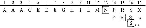
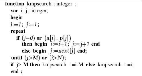
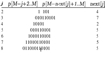
19. String Searching . . . 241 A Short History, Brute-Force Algorithm, Knuth-Morris-Pratt Algorzthm,
Bayer-Moore Algorithm, Rabin-Karp Algorithm, Multiple Searches
20. Pattern Matching . . . 257 Describing Patterns, Pattern Matching Machznes, Representzng
the Machine, Simulating the Machine
21. Parsing , . . . 269 Conteti-Free Grammars, Top-Down Parsing, Bottom-Up Parsing,
Compilers, Compiler-Compilers
22. File Compression . . . 283 Run-Length Encoding, Variable-Length Encoding
23. Cryptology . . . 295 Rules of the Game, Simple Methods, Encrypt:!on/Decryption
Machines, Publzc-Key Cryptosystems
G E O M E T R I C A L G O R I T H M S
24. Elementary Geometric Methods . . . 307 Poznts, Lines, and Polygons, Line Intersection, Simple
Closed Path, Inclusaon in 4 Polygon, Perspective
25. Finding the Convex Hull . . . 321 Rules of the Game, Package Wrapping, The Graham Scan,
Hull Selection, Performance Issues
26. Range Searching . . . 335 Elementary Methods, Grad Method, 2D Trees,
Multidimensaonal Range Searching
27. Geometric Intersection . , . . . 349 Horizontal and Vertical Lines, General Line Intersection
V l l l
GRAPH ALGORITHMS
29. Elementary Graph Algorithms . . . . Glossary, Representation, Depth-First Search, Mazes, Perspectzve
30. Connectivity . . . . Biconnectivity, Graph Traversal Algorzthms, Union-Find Algorithms 31. Weighted Graphs . . . .
Mmimum Spanning Tree, Shortest Path, Dense Graphs, Geometrzc Problems 32. Directed Graphs . . . .
Depth-Farst Search, Transitwe Closure, Topological Sorting, Strongly Connected Components
33. Network Flow . . . . The Network Flow Problem, Ford-Adkerson Method, Network Searching 34. Matching . . . , . . . . .
Bapartite Graphs, Stable Marriage Problem, Advanced Algorathms
ADVANCED TOPICS
35. Algorithm Machines . . . . General Approaches> Perfect ShujIes, Systolic Arrays
36. The Fast Fourier Transform . . . . Evaluate, M ultiply, Interpolate, Complez Roots of Unity, Evaluation at the Roots of Unity, Interpolatzon at the Roots of Unity, Implementation 37. Dynamic Programming . . . .
Knapsack Problem, Matriz Chain Product, Optimal Binary Search Trees, Shortest Paths, Time and Space Requirements
38. Linear Programming . . . . Lznear Programs, Geometric Interpretation, The Simplex Method,
Implementation
39. Exhaustive Search . . . . Exhaustive Search in Graphs, Backtrackzng, Permutation Generation, Approximation Algorithms
40. NP-complete Problems . . . . Deterministic and Nondeterministic Polynomial- Time Algorzthms,
NP-Completeness, Cook’ s Theorem, Some NP-Complete Problems
. . 3 7 3
. . 3 8 9
. . 4 0 7
. 4 2 1
. . 4 3 3
. . 4 4 3
. . 4 5 7
. . 4 7 1
. . 4 8 3
. . 4 9 7
. . 5 1 3
... ... ... ... ... : ... :... : ... :... : : ... ... : ... ... . ...:... :...: ...:...:... : : : : ...: ...:...: .... :
: : .... : .:.‘:.. . : : : .. : .... I .... .
.. ...
... .:: ‘LE.
-. * ... . :: : : : .... .... . . ... :... . ..: ....: ... :.: ... .:... : ... ... ....'...: .:...:..:...:. ... : ...: .... : ...: : -..: ... :... :...: :: :...: : : : ... :...: ... : .:. : .... :...: : ..:... :...:... : . ... . .:. ..:... :... . .::. : ... :... .:: . .:.. : ... : :..:. ...:. .: ...:... . . . . :..: :..: .:. : :. :.:. : .:..:-:. : .:. : :. :.:. . . . . -:.::.: : :: : :: . . . .. . * . . . :.:. . . . . : ::: .:: : :. :-:-. . . . . . . . . . . . . :. :.::: :. : .:: : :. : :..: :. : :*. :.:. :-:. . . . *.. . . . . . :. . : . :. :: . :. . : . :. : : . :... : . ::. :. : :. : :. : :..: :. :-:. : :. : :. : :. : :. . . . ::.. . .:. ..:a: . . . .:. : . . . :..: ..:.. . . . * . . . *.. . :. : :. : :. : :. : ::: :. : :. :.:. : :. : :: ..:....: . .::. :.. :... : ..::. ..: . .:. ..::. :... . . . : . . . : . . . : .*. : . . . : . . . : . . . .*. : .*. : . . . . . . . . . . a:: . ..: . .:.*. . . . : :.. . . . . . . . ..: : . . . :.:.. :.... : . . . ..: : . . . : . . ::.. . . . :-. :*:. I
... :.a: ... : :: ..: ... : .... : .... . .:. : .:. : ... : .... : .:..: . ... ...... : .... :::.: :.: : *. : :.: :::.: :.: -... ... ... .:. : ... : :.:: ... : :: : .... : ... : .:. : : .. : :..: .... : . ... . .::.: ... :... ...:. . : .. : .... : ... ... : ..: .:. : ...: ... :...:... :...:...: ... : ....: :: : .
. I ,
Introduction
The objective of this book is to study a broad variety of important and useful algorithms: methods for solving problems which are suited for computer implementation. We’ll deal with many different areas of applica-tion, always trying to concentrate on “fundamental” algorithms which are important to know and interesting to stu.dy. Because of the large number of areas and algorithms to be covered, we won’t have room to study many of the methods in great depth. However, we will try to spend enough time on each algorithm to understand its essential characteristics and to respect its subtleties. In short, our goal is to learn a large number of the most impor-tant algorithms used on computers today, well enough to be able to use and appreciate them.
To learn an algorithm well, one must implement it. Accordingly, the best strategy for understanding the programs presented in this book is to implement and test them, experiment with variants, and try them out on real problems. We will use the Pascal programming language to discuss and implement most of the algorithms; since, however, we use a relatively small subset of the language, our programs are easily translatable to most modern programming languages.
INTRODUCTION
This book is divided into forty chapters which are organized into seven major parts. The chapters are written so that they can be read independently, to as great extent as possible. Generally, the first chapter of each part gives the basic definitions and the “ground rules” for the chapters in that part; otherwise specific references make it clear when material from an earlier chapter is required.
Algorithms
When one writes a computer program, one is generally implementing a method of solving a problem which has been previously devised. This method is often independent of the particular computer to be used: it’s likely to be equally appropriate for many computers. In any case, it is the method, not the computer program itself, which must be studied to learn how the problem is being attacked. The term algorithm is universally used in computer science to describe problem-solving methods suitable for implementation as computer programs. Algorithms are the “stuff” of computer science: they are central objects of study in many, if not most, areas of the field.
Most algorithms of interest involve complicated methods of organizing the data involved in the computation. Objects created in this way are called data structures, and they are also central objects of study in computer science. Thus algorithms and data structures go hand in hand: in this book we will take the view that data structures exist as the byproducts or endproducts of algorithms, and thus need to be studied in order to understand the algorithms. Simple algorithms can give rise to complicated data structures and, conversely, complicated algorithms can use simple data structures.
When a very large computer program is to be developed, a great deal of effort must go into understanding and defining the problem to be solved, managing its complexity, and decomposing it into smaller subtasks which can be easily implemented. It is often true that many of the algorithms required after the decomposition are trivial to implement. However, in most cases there are a few algorithms the choice of which is critical since most of the system resources will be spent running those algorithms. In this book, we will study a variety of fundamental algorithms basic to large programs in many applications areas.
INTRODUCTION 5
to perform effectively on specific tasks, so that the opportunity to reimplement basic algorithms frequently arises.
Computer programs are often overoptimized. It may be worthwhile to take pains to ensure that an implementation is the most efficient possible only if an algorithm is to be used for a very large task or is to be used many times. In most situations, a careful, relatively simple implementation will suffice: the programmer can have some confidence that it will work, and it is likely to run only five or ten times slower than the best possible version, which means that it may run for perhaps an extra fraction of a second. By contrast, the proper choice of algorithm in the first place can make a difference of a factor of a hundred or a thousand or more, which translates to minutes, hours, days or more in running time. In this book, -we will concentrate on the simplest reasonable implementations of the best algorithms.
Often several different algorithms (or implementations) are available to solve the same problem. The choice of the very best algorithm for a particular task can be a very complicated process, often involving sophisticated mathe-matical analysis. The branch of computer science where such questions are studied is called analysis of algorithms. Many of the algorithms that we will study have been shown to have very good performance through analysis, while others are simply known to work well through experience. We will not dwell on comparative performance issues: our goal is to learn some reasonable algo-rithms for important tasks. But we will try to be aware of roughly how well these algorithms might be expected to perform.
Outline of Topics
Below are brief descriptions of the major parts of the book, which give some of the specific topics covered as well as some indication of the general orientation towards the material described. This set of topics is intended to allow us to cover as many fundamental algorithms as possible. Some of the areas covered are “core” computer science areas which we’ll study in some depth to learn basic algorithms of wide applicability. We’ll also touch on other disciplines and advanced fields of study within computer science (such as numerical analysis, operations research, clompiler construction, and the theory of algorithms): in these cases our treatment will serve as an introduction to these fields of study through examination of some basic methods.
6 IiVTRODUCTIOiV
and integration. The emphasis is on algorithmic aspects of the methods, not the mathematical basis. Of course we can’t do justice to advanced topics with this kind of treatment, but the simple methods given here may serve to introduce the reader to some advanced fields of study.
SORTING methods for rearranging files into order are covered in some depth, due to their fundamental importance. A variety of methods are devel-oped, described, and compared. Algorithms for several related problems are treated, including priority queues, selection, and merging. Some of these algorithms are used as the basis for other algorithms later in the book.
SEARCHING methods for finding things in files are also of fundamental importance. We discuss basic and advanced methods for searching using trees and digital key transformations, including binary search trees, balanced trees, hashing, digital search trees and tries, and methods appropriate for very large files. These methods are related to each other and similarities to sorting methods are discussed.
STRING PROCESSING algorithms include a range of methods for deal-ing with (long) sequences of characters. Strdeal-ing searchdeal-ing leads to pattern matching which leads to parsing. File compression techniques and cryptol-ogy are also considered. Again, an introduction to advanced topics is given through treatment of some elementary problems which are important in their own right.
GEOMETRIC ALGORITHMS comprise a collection of methods for solv-ing problems involvsolv-ing points and lines (and other simple geometric objects) which have only recently come into use. We consider algorithms for finding the convex hull of a set of points, for finding intersections among geometric objects, for solving closest point problems, and for multidimensional search-ing. Many of these methods nicely complement more elementary sorting and searching methods.
GRAPH ALGORITHMS are useful for a variety of difficult and impor-tant problems. A general strategy for searching in graphs is developed and applied to fundamental connectivity problems, including shortest-path, min-imal spanning tree, network flow, and matching. Again, this is merely an introduction to quite an advanced field of study, but several useful and inter-esting algorithms are considered.
I N T R O D U C T I O N
71. Preview
To introduce the general approach that we’ll be taking to studying algorithms, we’ll examine a classic elementary problem: “Reduce a given fraction to lowest terms.” We want to write 213, not 416, 200/300, or 178468/ 267702. Solving this problem is equival.ent to finding the greatest common divisor (gcd) of the numerator and the denominator: the largest integer which divides them both. A fraction is reduced to lowest terms by dividing both numerator and denominator by their greatest common divisor.
Pascal
A concise description of the Pascal language is given in the Wirth and Jensen Pascal User M anual and Report that serves as the definition for the language. Our purpose here is not to repeat information from that book but rather to examine the implementation of a few simple algorithms which illustrate some of the basic features of the language and. the style that we’ll be using.
Pascal has a rigorous high-level syntax which allows easy identification of the main features of the program. The variables (var) and functions (function) used by the program are declared first, f~ollowed by the body of the program. (Other major program parts, not used in the program below which are declared before the program body are constants and types.) Functions have the same format as the main program except that they return a value, which is set by assigning something to the function name within the body of the function. (Functions that return no value are called procedures.)
The built-in function readln reads a. line from the input and assigns the values found to the variables given as arguments; writeln is similar. A standard built-in predicate, eof, is set to true when there is no more input. (Input and output within a line are possible with read, write, and eoln.) The declaration of input and output in the program statement indicates that the program is using the “standard” input and output &reams.
10 CHA PTER 1
To begin, we’ll consider a Pascal program which is essentially a transla-tion of the definitransla-tion of the concept of the greatest common divisor into a programming language.
program example(input, output); var x, y: integer;
function gcd( u, v: integer) : integer; var t: integer;
begin
if u<v then t:=u else t:=v;
while (u mod t<>O) or (vmod t<>O) do t:=t-1; gcd:=t
end ; begin
while not eof do begin
readln (x, y ) ;
writeln(x, y, gcd(abs(x), abs(y))); end
end.
The body of the program above is trivial: it reads two numbers from the input, then writes them and their greatest common divisor on the output. The gcd function implements a “brute-force” method: start at the smaller of the two inputs and test every integer (decreasing by one until 1 is reached) until an integer is found that divides both of the inputs. The built-in function abs is used to ensure that gcd is called with positive arguments. (The mod function is used to test whether two numbers divide: u mod v is the remainder when u is divided by v, so a result of 0 indicates that v divides u.)
Many other similar examples are given in the Pascal User Manual and Report. The reader is encouraged to scan the manual, implement and test some simple programs and then read the manual carefully to become reason-ably comfortable with most of the features of Pascal.
Euclid’ s A lgorithm
PREVIEW 11
exactly the same as the remainder left after dividing u by v, which is what the mod function computes: the greatee:t common divisor of u and v is the same as the greatest common divisor of 1) and u mod v. If u mod v is 0, then v divides u exactly and is itself their greatest common divisor, so we are done. This mathematical description explains how to compute the greatest common divisor of two numbers by computing the greatest common divisor of two smaller numbers. We can implement this method directly in Pascal simply by having the gcd function call itself with smaller arguments:
function gcd( u, v:integer) : integer; begin
if v=O then gcd:= u
else gcd:=gcd(v, u mod v) end;
(Note that if u is less than v, then u m’od v is just u, and the recursive call just exchanges u and v so things work as described the next time around.) If the two inputs are 461952 and 116298, then the following table shows the values of u and v each time gcd is invoked:
(461952,1:16298) (116298,1:13058) (113058,324O)
(3240,2898) (2898,342) (342,162)
(162,18) (1% 0)
It turns out that this algorithm always uses a relatively small number of steps: we’ll discuss that fact in some moire detail below.
Recursion
A fundamental technique in the design of efficient algorithms is recursion:
12 CHAPTER 1
something else. This seems an obvious point when stated, but it’s probably the most common mistake in recursive programming. For similar reasons, one shouldn’t make a recursive call for a larger problem, since that might lead to a loop in which the program attempts to solve larger and larger problems.
Not all programming environments support a general-purpose recursion facility because of intrinsic difficulties involved. Furthermore, when recursion is provided and used, it can be a source of unacceptable inefficiency. For these reasons, we often consider ways of removing recursion. This is quite easy to do when there is only one recursive call involved, as in the function above. We simply replace the recursive call with a goto to the beginning, after inserting some assignment statements to reset the values of the parameters as directed by the recursive call. After cleaning up the program left by these mechanical transformations, we have the following implementation of Euclid’s algorithm:
function gcd(u, v:integer):integer;
var t: integer;
begin
while v<>O do
begin t:= u mod v; u:=v; v:=t end;
gcd:=u
end ;
Recursion removal is much more complicated when there is more than one recursive call. The algorithm produced is sometimes not recognizable, and indeed is very often useful as a di.fferent way of looking at a fundamental al-gorithm. Removing recursion almost always gives a more efficient implemen-tation. We’ll see many examples of this later on in the book.
Analysis of Algorithms
In this short chapter we’ve already seen three different algorithms for the same problem; for most problems there are many different available algorithms. How is one to choose the best implementation from all those available?
This is actually a well developed area of study in computer science. Frequently, we’ll have occasion to call on research results describing the per-formance of fundamental algorithms. However, comparing algorithms can be challenging indeed, and certain general guidelines will be useful.
expected to take on “typical” input data, and in the worst case, the amount of time a program would take on the worst possible input configuration.
Many of the algorithms in this book are very well understood, to the point that accurate mathematical formulas are known for the average- and worst-case running time. Such formulas are developed first by carefully studying the program, to find the running time in terms of fundamental mathematical quantities and then doing a mathematical analysis of the quantities involved. For some algorithms, it is easy to hgure out the running time. For ex-ample, the brute-force algorithm above obviously requires min(u, VU)-gcd(u, V) iterations of the while loop, and this quantity dominates the running time if the inputs are not small, since all the other statements are executed either 0 or 1 times. For other algorithms, a substantial amount of analysis is in-volved. For example, the running time of the recursive Euclidean algorithm obviously depends on the “overhead” required for each recursive call (which can be determined only through detailed1 knowledge of the programming en-vironment being used) as well as the number of such calls made (which can be determined only through extremely sophisticated mathematical analysis). Several important factors go into this analysis which are somewhat out-side a given programmer’s domain of influence. First, Pascal programs are translated into machine code for a given computer, and it can be a challenging task to figure out exactly how long even one Pascal statement might take to execute (especially in an environment where resources are being shared, so that even the same program could have varying performance characteristics). Second, many programs are extremely sensitive to their input data, and per-formance might fluctuate wildly depending on the input. The average case might be a mathematical fiction that is not representative of the actual data on which the program is being used, and the worst case might be a bizarre construction that would never occur in practice. Third, many programs of interest are not well understood, and specific mathematical results may not be available. Finally, it is often the case that programs are not comparable at all: one runs much more efficiently on one particular kind of input, the other runs efficiently under other circumstances.
With these caveats in mind, we’ll use rough estimates for the running time of our programs for purposes of classification, secure in the knowledge that a fuller analysis can be done for important programs when necessary. Such rough estimates are quite often easy to obtain via the old programming saw “90% of the time is spent in 10% of the code.” (This has been quoted in the past for many different values of “go%.“)
CHAPTER 1
control structure of a program, that absorb all of the machine cycles. It is always worthwhile for the programmer to be aware of the inner loop, just to be sure that unnecessary expensive instructions are not put there.
Second, some analysis is necessary to estimate how many times the inner loop is iterated. It would be beyond the scope of this book to describe the mathematical mechanisms which are used in such analyses, but fortunately the running times many programs fall into one of a few distinct classes. When possible, we’ll give a rough description of the analysis of the programs, but it will often be necessary merely to refer to the literature. (Specific references are given at the end of each major section of the book.) For example, the results of a sophisticated mathematical argument show that the number of recursive steps in Euclid’s algorithm when u is chosen at random less than v is approximately ((12 In 2)/7r2) 1 n TJ. Often, the results of a mathematical analysis are not exact, but approximate in a precise technical sense: the result might be an expression consisting of a sequence of decreasing terms. Just as we are most concerned with the inner loop of a program, we are most concerned with the leading term (the largest term) of a mathematical expression.
As mentioned above, most algorithms have a primary parameter N, usually the number of data items to be processed, which affects the running time most significantly. The parameter N might be the degree of a polyno-mial, the size of a file to be sorted or searched, the number of nodes in a graph, etc. Virtually all of the algorithms in this book have running time proportional to one of the following functions:
1 Most instructions of most programs are executed once or at most only a few times. If all the instructions of a program have this property, we say that its running time is constant. This is obviously the situation to strive for in algorithm design.
log N When the running time of a program is logarithmic, the program gets slightly slower as N grows.This running time commonly occurs in programs which solve a big problem by transforming it into a smaller problem by cutting the size by some constant fraction. For our range of interest, the running time can be considered to be less than a Yarge” constant. The base of the logarithm changes the constant, but not by much: when N is a thousand, log N is 3 if the base is 10, 10 if the base is 2; when N is a million, 1ogN is twice as great. Whenever N doubles, log N increases by a constant, but log N doesn’t double until N increases to N2.
PREVTEW 15
doubles, then so does the running time. This is the optimal situation for an algorithm that must process N inputs (or produce N outputs). NlogN This running time arises in algorithms which solve a problem by
N2
N3
2N
breaking it up into smaller subpr’oblems, solving them independently, and then combining the solutions. For lack of a better adjective (linearithmic?), we’ll say that th’e running time of such an algorithm is “N log N.” When N is a million, N log N is perhaps twenty million. When N doubles, the running time more than doubles (but not much more).
When the running time of an algorithm is quadratic, it is practical for use only on relatively small problems. Quadratic running times typically arise in algorithms which process all pairs of data items (perhaps in a double nested loop). When N is a thousand, the running time is a million. Whenever N doubles, the running time increases fourfold.
Similarly, an algorithm which prlocesses triples of data items (perhaps in a triple-nested loop) has a cubic running time and is practical for use only on small problems. VVhen N is a hundred, the running time is a million. Whenever N doubles, the running time increases eightfold.
Few algorithms with exponential running time are likely to be ap-propriate for practical use, though such algorithms arise naturally as “brute-force” solutions to problems. When N is twenty, the running time is a million. Whenever N doubles, the running time squares!
The running time of a particular prlogram is likely to be some constant times one of these terms (the “leading term”) plus some smaller terms. The values of the constant coefficient and the terms included depends on the results of the analysis and on implementation details. Roughly, the coefficient of the leading term has to do with the number of instructions in the inner loop: at any level of algorithm design it’s prudent to limit the number of such instructions. For large N the effect of the leading term dominates; for small N or for carefully engineered algorithms, more terms may contribute and comparisions of algorithms are more difficult. In most cases, we’ll simply refer to the running time of programs as “linear,” “N log N, ” “cubic,” etc., with the implicit understanding that more detailed analysis or empirical studies must be done in cases where efficiency is very important.
CHAPTER 1
of these functions should be considered to be much closer to N log N than to N2 for large N.
One further note on the “log” function. As mentioned above, the base of the logarithm changes things only by a constant factor. Since we usually deal with analytic results only to within a constant factor, it doesn’t matter much what the base is, so we refer to “logN,” etc. On the other hand, it is sometimes the case that concepts can be explained more clearly when some specific base is used. In mathematics, the natz~ral logarithm (base e = 2.718281828.. .) arises so frequently that a special abbreviation is commonly used: log, N = In N. In computer science, the binary logarithm (base 2) arises so frequently that the abbreviation log, N = lg N is commonly used. For example, lg N rounded up to the nearest integer is the number of bits required to represent N in binary.
Implementing Algorithms
The algorithms that we will discuss in this book are quite well understood, but for the most part we’ll avoid excessively detailed comparisons. Our goal will be to try to identify those algorithms which are likely to perform best for a given type of input in a given application.
The most common mistake made in the selection of an algorithm is to ignore performance characteristics. Faster algorithms are often more compli-cated, and implementors are often willing to accept a slower algorithm to avoid having to deal with added complexity. But it is often the case that a faster algorithm is really not much more complicated, and dealing with slight added complexity is a small price to pay to avoid dealing with a slow algorithm. Users of a surprising number of computer systems lose substantial time waiting for simple quadratic algorithms to finish when only slightly more complicated N log N algorithms are available which could run in a fraction the time.
PREVIEW 17
1 8
Exercises
1.
2.
3.
4.
5.
6.
7.
8.
9.
10.
Solve our initial problem by writing a Pascal program to reduce a given fraction x/y to lowest terms.
Check what values your Pascal system computes for u mod v when u and v are not necessarily positive. Which versions of the gcd work properly when one or both of the arugments are O?
Would our original gcd program ever be faster than the nonrecursive version of Euclid’s algorithm?
Give the values of u and v each time the recursive gcd is invoked after the initial call gcd(12345,56789).
Exactly how many Pascal statements are executed in each of the three gcd implementations for the call in the previous exercise?
Would it be more efficient to test for u>v in the recursive implementation of Euclid’s algorithm?
Write a recursive program to compute the largest integer less than log, N based on the fact that the value of this function for N div 2 is one greater than for N if N > 1.
Write an iterative program for the problem in the previous exercise. Also, write a program that does the computation using Pascal library sub-routines. If possible on your computer system, compare the performance of these three programs.
Write a program to compute the greatest common divisor of three integers u, v, and w.
19
SOURCES for background material
A reader interested in learning more about Pascal will find a large number of introductory textbooks available, for example, the ones by Clancy and Cooper or Holt and Hune. Someone with experience programming in other languages can learn Pascal effectively directly from the manual by Wirth and Jensen. Of course, the most important thing to do to learn about the language is to implement and debug as many programs as possible.
Many introductory Pascal textbooks contain some material on data struc-tures. Though it doesn’t use Pascal, an important reference for further infor-mation on basic data structures is volume one of D.E. Knuth’s series on The Art of Computer Programming. Not only does this book provide encyclopedic coverage, but also it and later books in the series are primary references for much of the material that we’ll be covering in this book. For example, anyone interested in learning more about Euclid’s algorithm will find about fifty pages devoted to it in Knuth’s volume two.
Another reason to study Knuth’s volume one is that it covers in detail the mathematical techniques needed for the analysis of algorithms. A reader with little mathematical background sh’ould be warned that a substantial amount of discrete mathematics is required to properly analyze many algo-rithms; a mathematically inclined reader will find much of this material ably summarized in Knuth’s first book and applied to many of the methods we’ll be studying in later books.
M. Clancy and D. Cooper, Oh! Pascal, W. W. Norton & Company, New York, 1982.
R. Holt and J. P.Hume, Programming Standard Pascal, Reston (Prentice-Hall), Reston, Virginia, 1980.
D. E. Knuth, The Art of Computer Programming. Volume 1: Fundamental
Algorithms, Addison-Wesley, Reading, MA, 1968.
D. E. Knuth, The Art of Computer Programming. Volume .2: Seminumerical
Algorithms, Addison-Wesley, Reading, MA, Second edition, 1981.
MATHEMATICAL ALGORITHMS
5 *.a . .). . . . . . .I -. .
. . . -.- “. -.. . . m..‘.’ l .’ : -. :- -.: -.. : .:. . .. :
--- a-:.. . * . . ..‘..- a.-*. . . . ‘.:. . . . . .
; . i . . . . .+. .
-, ,.- . . . . . , . . .: . : mm. . . . : . *’. . c -*.,
- . .- 5. - - /: .m-. . . .- - .l . .
.- . . - -. - . . 5
2. Arithmetic
cl
Algorithms for doing elementary arithmetic operations such as addition, multiplication, and division have a. very long history, dating back to the origins of algorithm studies in the work of the Arabic mathematician al-Khowdrizmi, with roots going even further back to the Greeks and the Babylonians.Though the situation is beginning to change, the raison d’e^tre of many computer systems is their capability for doing fast, accurate numerical cal-culations. Computers have built-in capabilities to perform arithmetic on in-tegers and floating-point representations of real numbers; for example, Pascal allows numbers to be of type integer or re;d, with all of the normal arithmetic operations defined on both types. Algorithms come into play when the opera-tions must be performed on more complicated mathematical objects, such as polynomials or matrices.
In this section, we’ll look at Pascal implementations of some simple algorithms for addition and multiplication of polynomials and matrices. The algoritms themselves are well-known and straightforward: we'll be examining
sophisticated algorithms for these problems in Chapter 4. Our main purpose in this section is to get used to treating th’ese mathematical objects as objects for manipulation by Pascal programs. This translation from abstract data to something which can be processed by a computer is fundamental in algorithm design. We’ll see many examples throughout this book in which a proper representation can lead to an efficient algorithm and vice versa. In this chapter, we’ll use two fundamental ways of structuring data, the array and the linked list. These data structures are used by many of the algorithms in this book; in later sections we’ll study some more advanced data structures.
Polynomials
Suppose that we wish to write a program that adds two polynomials: we would
2 4 CJUJ’TER 2
like it to perform calculations like
(1+ 2x - 3x3) + (2 -x) = 3 + x - 3x3.
In general, suppose we wish our program to be able to compute r(x) = p(x) +
q(x), where p and q are polynomials with N coefficients. The following program is a straightforward implementation of polynomial addition:
program poJyadd(input, output);
con& maxN=lOO;
var p, q, r: array [ O..maxN] of real; N, i: integer;
begin readln (N) ;
for i:=O to N-l do read(p[i]); for i:=O to N-l do read(q[i]);
for i:=O to N-J do r[i] :=p[i]+q[i];
for i:=O to N-l do write(r[i]);
wri teln end.
In this program, the polynomial p(z) = pc + pix + a.. + pr\r-isN-’ is represented by the array p [O..N-l] with p [j] = pj, etc. A polynomial of degree N-l is defined by N coefficients. The input is assumed to be N, followed by the p coefficients, followed by the q coefficients. In Pascal, we must decide ahead of time how large N might get; this program will handle polynomials up to degree 100. Obviously, maxN should be set to the maximum degree anticipated. This is inconvenient if the program is to be used at different times for various sizes from a wide range: many programming environments allow “dynamic arrays” which, in this case, could be set to the size N. We’ll see another technique for handling this situation below.
The program above shows that addition is quite trivial once this repre-sentation for polynomials has been chosen; other operations are also easily coded. For example, to multiply we can replace the third for loop by
for i:=O to 2*(N-I) do r[i] :=O; for i:=O to N-l do
for j:=O to N-l do
ARITHMETIC
Also, the declaration of r has to be suita.bly changed to accomodate twice as many coefficients for the product. Each of the N coefficients of p is multiplied by each of the N coefficients of q, so this is clearly a quadratic algorithm.
An advantage of representing a polynomial by an array containing its coefficients is that it’s easy to reference any coefficient directly; a disadvantage is that space may have to be saved for more numbers than necessary. For example, the program above couldn’t reasonably be used to multiply
(1+ .10000)(1+ 2,lOOOO) = 1+ 3~10000 + 2~20000,
even though the input involves only four c’oefficients and the output only three. An alternate way to represent a pol:ynomial is to use a linked list. This involves storing items in noncontiguous memory locations, with each item containing the address of the next. The Pascal mechanisms for linked lists are somewhat more complicated than for arrays. For example, the following pro-gram computes the sum of two polynomials using a linked list representation (the bodies of the readlist and add functions and the writelist procedure are given in the text following):
program polyadd(input, output); type link q = mode;
node = record c: real; next: link end ; var N: integer; a: link;
function readlist(N: integer) : link; procedure writelist(r: link); function add(p, q: link) : link; begin
readln(N); new(z);
writelist(add(readlist(N), readlist(N end.
2 6 CHAPTER 2
it in a. (The other nodes on the lists processed by this program are created in the readlist and add routines.)
The procedure to write out what’s on a list is the simplest. It simply steps through the list, writing out the value of the coefficient in each node encountered, until z is found:
procedure writelist(r: link); begin
while r<>z do
begin write(rf.c); r:=rt.next end; wri teln
end ;
The output of this program will be indistinguishable from that of the program above which uses the simple array representation.
Building a list involves first calling new to create a node, then filling in the coefficient, and then linking the node to the end of the partial list built so far. The following function reads in N coefficients, assuming the same format as before, and constructs the linked list which represents the corresponding polynomial:
function readlist (N: integer) : link; var i: integer; t: link;
begin t:=z;
for i:=O to N-l do
begin new(tf.next); t:=tt.next; read(tt.c) end; tf.next:=z; readlist:=zf.next; zf.next:=z
end ;
The dummy node z is used here to hold the link which points to the first node on the list while the list is being constructed. After this list is built, a is set to link to itself. This ensures that once we reach the end of a list, we stay there. Another convention which is sometimes convenient, would be to leave z pointing to the beginning, to provide a way to get from the back to the front.
ARITHM73TIC 2 7
function add(p, q: link): link; var t : link ;
begin
t:=z;
repeat
new(tt.next); t:=tf.next; tf.c:=pt.c+qf.c;
p:=pf.next; q:=qf.next
until (p=z) and (q=z);
tt.next:=z; add:=zt.next
e n d ;
Employing linked lists in this way, we use only as many nodes as are required by our program. As N gets larger, we simply make more calls on new.
By itself, this might not be reason enough. to use linked lists for this program, because it does seem quite clumsy comlpared to the array implementation above. For example, it uses twice as much space, since a link must be stored along with each coefficient. However, as suggested by the example above, we can take advantage of the possibility that many of the coefficients may be zero. We can have list nodes represent only the nonzero terms of the polynomial by also including the degree of the term represented within the list node, so that each list node contains values of c and j to represent cxj. It is then convenient to separate out the function of creating a node and adding it to a list, as follows:
type link = fnode;
node = record c: real; j: integer; next: link end; function listadd(t: link; c: real; j: integer): link;
begin
new(tf.next); t:=tT.next; tf.c:=c; tt.j:=j;
listadd:=t;
end ;
28 CIZ4PTER 2
way, the list nodes might be kept in increasing order of degree of the term represented.
Now the add function becomes more interesting, since it has to perform an addition only for terms whose degrees match, and then make sure that no term with coefficient 0 is output:
function add(p, q: link): link; begin
t:=z; st.j:=iV+l; repeat
if (pf.j=qf.j) and (pf.c+qf.c<>O.O) then begin
t:=listadd(t,pf.c+qt.c,pt.j); p:=pt.next; q:=qf.next end
else if pf.j<qt.j then
begin t:=listadd(t, pt.c, pf.j); p:=pt.next end else if qf.j<pt.j then
begin t:=listadd(t, qf.c, q1.j); q:=qt.next end; until (p=z) and (q=z);
tf.next:=z; add:=zf.next end ;
These complications are worthwhile for processing “sparse” polynomials with many zero coefficients, but the array representation is better if there are only a few terms with zero coefficients. Similar savings are available for other operations on polynomials, for example multiplication.
Matrices
We can proceed in a similar manner to implement basic operations on two-dimensional matrices, though the programs become more complicated. Sup-pose that we want to compute the sum of the two matrices
ARITHMETIC 29
program matrixadd(input, output); const maxN=lO;
var p, q, r: array [O..maxN, O..maxN] of real; N, i, j: integer;
begin readln (N) ;
for i:=O to N-l do for j:=O to N-l do read(p[i, j]); for i:=O to N-l do for j:=O to N-l do read(q[i, j]);
for i:=O to N-l do for j:=O to N-l do r[i, j]:=p[i, j]+q[i, j]; for i:=O to N-l do for j:=O to N do
if j=N then writeln else write(r[i, j]); end.
Matrix multiplication is a more complicated operation. For our example,
Element r[i, j] is the dot product of the ith row of p with the jth column of q. The dot product is simply the sum of the N term-by-term multiplica-tions p[i, l]*q[l, j]+p[i, 2]*q[2, j]+... p[i, N-l]*q[N-I, j] as in the following program:
for i:=O to h-1 do for j:=O to N-l do
begin t:=o.o;
for k:=iO to N-l do t:=t+p[i, k]*q[k, j]; r[i, j]:=t
end ;
Each of the N2 elements in the result matrix is computed with N mul-tiplications, so about N3 operations are required to multiply two N by N matrices together. (As noted in the previous chapter, this is not really a cubic algorithm, since the number of data items in this case is about N2, not N.)
CHAPTER 2
matrices represented in this way is similar to our implementation for sparse polynomials, but is complicated by the fact that each node appears on two lists.
Data Structures
Even if there are no terms with zero coefficients in a polynomial or no zero elements in a matrix, an advantage of the linked list representation is that we
don’t need to know in advance how big the objects that we’ll be processing are. This is a significant advantage that makes linked structures preferable in many situations. On the other hand, the links themselves can consume a significant part of the available space, a disadvantage in some situations. Also, access to individual elements in linked structures is much more restricted than in arrays.
We’ll see examples of the use of these data structures in various algo-rithms, and we’ll see more complicated data structures that involve more constraints on the elements in an array or more pointers in a linked repre-sentation. For example, multidimensional arrays can be defined which use multiple indices to access individual items. Similarly, we’ll encounter many “multidimensional” linked structures with more than one pointer per node. The tradeoffs between competing structures are usually complicated, and different structures turn out to be appropriate for different situations.
AFUTHAJETIC 31
Exercises
1.
2.
3.
4.
5.
6.
7.
8.
9.
10.
Another way to represent polynomials is to write them in the form rc(x-rr)(z - r2) . . . (X - TN). How would you multiply two polynomials in this representation?
How would you add two polynomials represented as in Exercise l?
Write a Pascal program that multiplies two polynomials, using a linked list representation with a list node for each term.
Write a Pascal program that multiplies sparse polynomials, using a linked list representation with no nodes for terms with 0 coefficients.
Write a Pascal function that returns the value of the element in the ith row and jth column of a sparse matrix, assuming that the matrix is represented using a linked list representation with no nodes for 0 entries.
Write a Pascal procedure that sets the value of the element in the ith row and jth column of a sparse matrix to v, assuming that the matrix is represented using a linked list representation with no nodes for 0 entries.
What is the running time of matrix multiplication in terms of the number of data items?
Does the running time of the polynornial addition programs for nonsparse input depend on the value of any of the coefficients?
Run an experiment to determine which of the polynomial addition pro grams runs fastest on your computer system, for relatively large N.
3. Random Numbers
Our next set of algorithms will bie methods for using a computer to generate random numbers. We will find many uses for random numbers later on; let’s begin by trying to get a better idea of exactly what they are.
Often, in conversation, people use the term random when they really mean arbitrary. When one asks for an trrbitrary number, one is saying that one doesn’t really care what number one gets: almost any number will do. By contrast, a random number is a precisely defined mathematical concept: every number should be equally likely to occur. A random number will satisfy
someone who needs an arbitrary number, but not the other way around. For “every number to be equally likely to occur” to make sense, we must restrict the numbers to be used to some finite domain. You can’t have a random integer, only a random integer in some range; you can’t have a random real number, only a random fraction in some range to some fixed precision.
It is almost always the case that not just one random number, but a
sequence of random numbers is needed (otherwise an arbitrary number might do). Here’s where the mathematics comes in: it’s possible to prove many facts about properties of sequences of random numbers. For example, we can expect to see each value about the same number of times in a very long sequence of random numbers from a small domain. Random sequences model many natural situations, and a great deal is known about their properties. To be
consistent with current usage, we’ll refer to numbers from random sequences as random numbers.
There’s no way to produce true random numbers on a computer (or any deterministic device). Once the program is written, the numbers that it will produce can be deduced, so how could they be random? The best we can hope to do is to write programs which produce isequences of numbers having many of the same properties as random numbers. Such numbers are commonly called pseudo-random numbers: they’re not really random, but they can be useful
CHAF’ TER 3
as approximations to random numbers, in much the same way that floating-point numbers are useful as approximations to real numbers. (Sometimes it’s convenient to make a further distinction: in some situations, a few properties of random numbers are of crucial interest while others are irrelevant. In such situations, one can generate quasi-random numbers, which are sure to have the properties of interest but are unlikely to have other properties of random numbers. For some applications, quasi-random numbers are provably preferable to pseudo-random numbers.)
It’s easy to see that approximating the property “each number is equally likely to occur” in a long sequence is not enough. For example, each number in the range [l,lOO] appears once in the sequence (1,2,. . . ,lOO), but that sequence is unlikely to be useful as an approximation to a random sequence. In fact, in a random sequence of length 100 of numbers in the range [l,lOO], it is likely that a few numbers will appear more than once and a few will not appear at all. If this doesn’t happen in a sequence of pseudo-random numbers, then there is something wrong with the random number generator. Many sophisticated tests based on specific observations like this have been devised for random number generators, testing whether a long sequence of pseudo random numbers has some property that random numbers would. The random number generators that we will study do very well in such tests.
We have been (and will be) talking exclusively about uniform random numbers, with each value equally likely. It is also common to deal with random numbers which obey some other distribution in which some values are more likely than others. Pseudo-random numbers with non-uniform distributions are usually obtained by performing some operations on uniformly distributed ones. Most of the applications that we will be studying use uniform random numbers.
Applications
Later in the book we will meet many applications in which random numbers will be useful. A few of them are outlined here. One obvious application is in
cryptography, where the major goal is to encode a message so that it can’t be read by anyone but the intended recipient. As we will see in Chapter 23, one way to do this is to make the message look random using a pseudo-random sequence to encode the message, in such a way that the recipient can use the same pseudorandom sequence to decode it.
RANDOM NUM BERS 3 5
When a very large amount of data is to be analyzed, it is sometimes sufficient to process only a very small amount of the data, chosen according to random sampling. Such applications are widespread, the most prominent being national political opinion polls.
Often it is necessary to make a choice when all factors under consideration seem to be equal. The national draft lottery of the 70’s or the mechanisms used on college campuses to decide which students get the choice dormitory rooms are examples of using random numbers for decision making. In this way, the responsibility for the decision is given to “fate” (or the computer).
Readers of this book will find themselves using random numbers exten-sively for simulation: to provide random or arbitrary inputs to programs. Also, we will see examples of algorithms which gain efficiency by using random numbers to do sampling or to aid in decision making.
Linear Co ngruential M etho d
The most well-known method for generating random numbers, which has been used almost exclusively since it was introduced by D. Lehmer in 1951, is the so-called linear congruential method. If a [I] contains some arbitrary number, then the following statement fills up an array with N random numbers using this method:
for i:=2 to N do
a[i]:=(a[i-l]*b $1) mod m
That is, to get a new random number, take the previous one, multiply it by a constant b, add 1 and take the remainder when divided by a second constant m. The result is always an integer between 0 and m-l. This is attractive for use on computers because the mod function is usually trivial to implement: if we ignore overflow on the arithmetic operations, then most com-puter hardware will throw away the bits that overflowed and thus effectively perform a mod operation with m equal to one more than the largest integer that can be represented in the computer word.
Simple as it may seem, the linear congruential random number generator has been the subject of volumes of detailed and difficult mathematical analysis. This work gives us some guidance in choosing the constants b and m. Some
CHAPTER 3
b should be an arbitrary constant with no particular pattern in its digits,
except that it should end with *-~21, with z even: this last requirement is admittedly peculiar, but it prevents the occurrence of some bad cases that have been uncovered by the mathematical analysis.
The rules described above were developed by D.E.Knuth, whose textbook covers the subject in some detail. Knuth shows that these choices will make the linear congruential method produce good random numbers which pass several sophisticated statistical tests. The most serious potential problem, which can become quickly apparent, is that the generator could get caught in a cycle and produce numbers it has already produced much sooner than it should. For example, the choice b=l9, m=381, with a[ I] =O, produces the sequence 0,1,20,0,1,20 ,..., a notrvery-random sequence of integers between 0 and 380.
Any initial value can be used to get the random number generator started with no particular effect except of course that different initial values will give rise to different random sequences. Often, it is not necessary to store the whole sequence as in the program above. Rather, we simply maintain a global variable a, initialized with some value, then updated by the computation
a:=(a*b+l) mod m.
In Pascal (and many other programming languages) we’re still one step away from a working implementation because we’re not allowed to ignore overflow: it’s defined to be an error condition that can lead to unpredictable results. Suppose that we have a computer with a 32-bit word, and we choose
m =190000000, b=3f 415821, and, initially, a=1234567. All of these values are comfortably less than the largest integer that can be represented, but the first a* b+l operation causes overflow. The part of the product that causes the overflow is not relevant to our computation, we’re only interested in the last eight digits. The trick is to avoid overflow by breaking the multiplication up into pieces. To multiply p by q, we write p = 104pr + pc and q = 104qr + qo,
so the product is
Pq= (104Pl + po)(104q1 + qo)
= lo8Plql + 104(p1qo + poq1) + poqo.
RAAJDOM NUMBERS 37
program random (inpu t, output) ;
con& m=100000000; ml=lOOOO; b=31415821; var i, a, IV: integer;
function mult(p, q: integer): integer; var pl, ~0, ql, q0: integer;
begin
pl :=p div ml ; pO:=p mod ml ; ql :=q div ml; qO:=q mod ml;
mult:=( ((pO*ql+pl*qO) mod ml)*ml+pO*qO) mod m; end ;
function random : integer ; begin
a:=(mult(a, b)+l) mod m; random :=a;
end ; begin read(hJ, a);
for i:=l to N do writeln(random) end.
The function mult in this program computes p*q mod m, with no overflow as long as m is less than half the largest integer that can be represented. The technique obviously can be applied with m=ml*ml for other values of ml.
Here are the ten numbers produced by this program with the input N = 10 and a = 1234567:
358845’08 80001069 63512650 43635651 1034472 87181513 6917174 209855 67115956 59939877
CHA PTER 3
not particularly random. This leads to a common and serious mistake in the use of linear congruential random number generators: the following is a bad program for producing random numbers in the range [0, r - 11:
function randombad(r: integer) : integer; begin
a:=(mult(b, a)+l) mod m;
randombad:=a mod r;
end ;
The non-random digits on the right are the only digits that are used, so the resulting sequence has few of the desired properties. This problem is easily fixed by using the digits on the left. We want to compute a number between 0 and r-l by computing a*r mod m, but, again, overflow must be circumvented, as in the following implementation:
function randomint(r: integer): integer; begin
a:=(mult(a, b)+l) mod m;
randomint:=((a div ml)*r) div ml
end ;
Another common technique is to generate random real numbers between 0 and 1 by treating the above numbers as fractions with the decimal point to the left. This can be implemented by simply returning the real value a/m rather than the integer a. Then a user could get an integer in the range [O,r) by simply multiplying this value by r and truncating to the nearest integer. Or, a random real number between 0 and 1 might be exactly what is needed.
A dditive Congruential M ethod
RANDOM NUMBERS 39
Below are listed the contents of the register for the first sixteen steps of the process:
0 1 2 3 4 5 6 7 1011 0101 1010 1101 1110 1111 0111 0011
8 9 10 11 12 13 14 15 0001 1000 0100 0010 1001 1100 0110 1011
Notice that all possible nonzero bit patterns occur, the starting value repeats after 15 steps. As with the linear congruential method, the mathe-matics of the properties of these registers has been studied extensively. For example, much is known about the choices of “tap” positions (the bits used for feedback) which lead to the generation of all bit patterns for registers of various sizes.
Another interesting fact is that the calculation can be done a word at a time, rather than a bit at a time, according to the same recursion formula. In our example, if we take the bitwise “exclusive or” of two successive words, we get the word whic