•Theconceptofpointersandtheirusewithdifferentdatatypes •
For your convenience Apress has placed some of the front
matter material after the index. Please use the Bookmarks
v
Contents at a Glance
About the Authors ...
xiii
Acknowledgments ...
xv
Introduction ...
xvii
Chapter 1: Memory, Runtime Memory Organization, and Virtual Memory
■
...
1
Chapter 2: Pointer Basics
■
...
27
Chapter 3: Pointer Arithmetic and Single Dimension Arrays
■
...
43
Chapter 4: Pointers and Strings
■
...
57
Chapter 5: Pointers and Multidimensional Arrays
■
...
71
Chapter 6: Pointers to Structures
■
...
89
Chapter 7: Function Pointers
■
...
113
Chapter 8: Pointers to File I/O
■
...
123
Introduction
Ever since the introduction of the C programming language in 1978,it has been regarded as a powerful language and has gained popularity among programmers worldwide. Despite starting as a language for the UNIX operating system, it has been used extensively in implementing wonderful and very complex software on multiple platforms. C has always been the default choice of language for writing any low level layers, device drivers, embedded system programming, programming mobile devices and so on.
One of most important features of C is pointers, which is an interesting topic and many times difficult to grasp. C being a relatively low level language, requires that programmers are well versed with many fundamental notions of computers while using it. And also, C is not a strongly-typed language.
The concept of pointer is known for its cryptic nature and that makes the understanding of it in some cases very difficult. This book is meant to provide an understanding of the concept of pointers for a novice or an intermediate or an expert programmer. To make the reader understand any concept of pointers we have provided back ground information which is not related to the language but which is part of the computer science literature. This background information will help the reader to understand the concepts very easily.
The book is organized as follows.
Chapter 1 is the basis for other chapters. It describes the concept of memory and runtime memory which provides the reader with an understanding of the basic concept of how memory is accessed and how data/ instructions are stored in memory. This chapter helps in understanding the compilation steps. This includes explanation of how intermediate results such as preprocessing, assembly and object code are generated. It also gives detailed background of how memory segments/sections are created by the compiler. Memory segments are explained in detail with pros and cons which will help readers to understand the usage of various kinds of variables. This chapter is also augmented with the understanding of the concept of virtual memory.
Chapter 2 introduces the concept of a pointer variable and the most important operations on it (referencing and dereferencing). This chapter explains the concept of initialization, comparison and memory allocation to pointer variables. It also explains the notion of a NULL pointer, dangling pointer, VOID pointer and CONST qualifiers. This chapter also explains the notion of how a pointer variable is used with different types of primitive data types such as integer, char and so on. This chapter also provides an explanation of how multilevel pointers can be used to access memory addresses and the values stored at those locations.
Chapter 3 contains a detailed explanation of pointer arithmetic and single dimensional arrays. Pointer arithmetic is explained in detailed. Explanation is given on how pointers can be used to access various contiguous memory locations using addition and subtraction operations on pointers. A section in this chapter explains the usage of pointers to access array data types. This chapter gives illustrious insight on how various kinds of expressions can be used to access a particular index of an array.
Chapter 4 contains an explanation of how pointers can be used to initialize static strings and manipulate them. Many examples have been included in the form of basic string manipulation functions such as strcpy, substring and so on. String manipulation is one of the most important requirements while solving and implementing algorithms.
xviii
Chapter 6 is about the detailed description of how structures and its member fields can be accessed with pointers. Usage of structures and pointers helps in implementing complex and dynamic data structures. Illustrious examples have been included in the chapter to explain the implementation of data structures such as linked lists and binary trees with the help of pointers. A section is also dedicated to explain how a function of a program can be accessed dynamically with the help of function pointers.
Chapter 7 is an explanation of usage of the function pointers concept.
Memory, Runtime Memory
Organization, and Virtual Memory
I have always wondered why the concept of a pointer is so dauntingly difficult to grasp. The concept of a pointer can be intuitively understood only if you are able to visualize it in your mind. By “visualizing” I mean being able to represent mentally its storage, lifespan, value, and so forth. Before getting into the nitty-gritty of pointers, however, you need to be equipped with the concepts of memory, runtime memory organization of the program, virtual memory, the execution model, and something of the assembly language.
This chapter introduces these prerequisite concepts by way of a generic case of how the modeling of runtime organization is done and some simple examples of how a CPU accesses the different sections of a process during runtime. Finally, it introduces the concept of virtual memory.
Subsequent chapters will go through the basics of pointers, their usage, advanced topics of pointer manipulation, and algorithms for manipulating memory addresses and values. The final chapters focus on practical applications.
The chapters are designed to be discrete and sequential, so you may skip any sections you are already familiar with.
Memory and Classification
Memory by definition is used to store sequences of instructions and data. Memory is classified to be permanent or temporary depending on its type. Throughout this work, references to memory are to be implicitly understood as meaning temporary/non-persistent storage (such as RAM, cache, registers, etc.), unless explicitly identified as permanent storage. Memory is formed as a group of units in which information is stored in binary form. The size of the group depends on the underlying hardware or architecture and its number varies (1, 2, 4, 8, 16, 32, 64, or 128 bit).
Classification
2
Let’s take a look at each of these different kinds of memory with respect to their usage and connectivity. Some of the memory could be present inside the chip (on-chip) along with processors, and some are attached to the ports on the motherboard. Communication or transfer of data takes place with the help of the address bus.
• Registers: These registers are mainly on the chip along with the processor. Depending on the architecture they vary in numbers. The descriptions below about registers are based on the Intel IA32 architecture.
• Segment Registers: CS, DS, ES, etc. These registers help in implementing support for segmentation and eventually to support multiprogrammed environments.
• System Registers: CR0, CR1, EFLAGS etc. These registers help in initializing and controlling system operations. Similarly, there are many other registers along with the ones mentioned above. I will not go into detail about each of the other registers.
• Caches: Typically, cache is high-speed memory that is used to store small portions of data temporarily. And probably this is the data that will be accessed frequently in the near future. In modern systems, caches also have some hierarchical structure.
L1 cache is faster and closer to the CPU but smaller in size. •
L2 cache is less fast and less close to the CPU but comparatively bigger in size. •
SRAM is used for cache memories as they are faster than DRAM. Also, there exist •
dedicated instruction cache and data cache in some architectures, such that instruction code will reside in the instruction cache while the data portion on which these
instructions work will reside in the data cache.
• Main Memory: In some literature the main memory is also called the physical memory. This is the place where all the data and instruction to be executed is loaded. When a program is executed, the operating system creates a process on its behalf in the main memory. I do not explain this process and its creation in this chapter, but I will do so in detail in subsequent chapters. The capacity of the main memory dictates the size of the software a system can handle. The size of the main memory runs in GBs. Also, the operating system shares part of the main memory along with other processes.
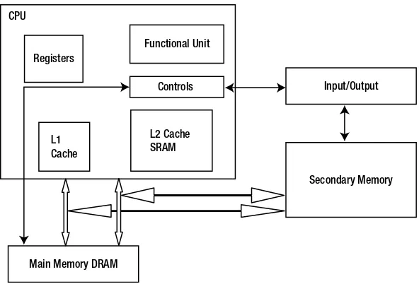
Now that you have a sense of the different kinds of memory in the system and what they do and contain, let’s see how they look when laid out and interconnected. Figure 1-2 schematically depicts a typical computer architecture and associated connectivity.
Type Capacity
Speed
(approx) Volatile/Nonvolatile Cost
Registers
16/32/64 bits, depending on
the type of CPU < 10ns Volatile
Cache in K bytes 10-50ns Volatile Increasing RAM (Main Memory) in Mbytes; some GBs 50-100ns Volatile
Secondary Storage in GBs and TBs 10 millisec Nonvolatile
Memory Layout
Memory is a linear array of locations, where each location has an address that is used to store the data at those locations. Figure 1-3 illustrates typical connectivity between the CPU and main memory.
CPU
Registers
Functional Unit
Controls
L1 Cache
L2 Cache SRAM
Main Memory DRAM
Input/Output
Secondary Memory
Figure 1-2. Memory hierarchy layout
CPU Memory
Controller
Main Memory
DRAM
Data Line Addr Line
Figure 1-3. Memory layout
4
Memory Address Data
Figure 1-4. Memory Dump
Figure 1-5. Data and instruction
How the Processor Accesses Main Memory
If we assume that a program is loaded into memory for execution, it is very important to understand how the CPU/ processor brings in all the instructions and data from these different memory hierarchies for execution. The data and instructions are brought into the CPU via the address and data bus. To make this happen, many units (the control unit, the memory controller, etc.) take part.
Data and Instruction
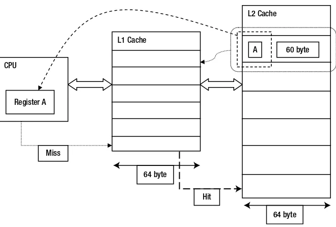
Let’s get into the details of how data is transferred into memory. Assume that the CPU is going to execute an instruction: mov eax, A. This assembly instruction moves the value stored at variable A to register eax. After the CPU decodes this instruction, it puts the address of variable A into the address bus and then this data is checked for whether it is present in the L1 cache. There can only be two cases: if the data is present, it is a hit; if it is not, it is a miss.
In case of a miss, the data is looked for in next level of hierarchy (i.e., L2 cache) and so on. If the data is a hit, the required data is copied to the register (the final destination), and it is also copied to the previous layer of hierarchy.
I will explain the copying of data, but first let’s look into the structure of cache memory and specifically into memory lines.
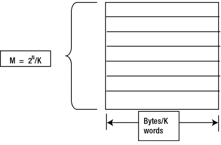
Cache Memory
In generic form, a cache has N lines of addressable (0 – 2N -1) units. Each line is capable of holding a certain amount of data in bytes (K words). In the cache world, each line is called a block. Cache views memory as an array of M blocks, where M = 2N/K, as shown in Figure 1-6. And the total cache size C = M* K .
Bytes/K words M = 2N/K
Figure 1-6. Cache memory model
Examples of realistic caches follow:
L1 cache = 32 KB and 64 B/line
L2 cache = 256 KB and 64 B/line
L3 cache = 4 MB and 64 B/line
Now you know a little about the structure of the cache, let’s analyze the hit and miss cache in two level of caches (L1 and L2). As noted in the discussion of the CPU executing the MOVL command, the CPU looks for the data in the L1 cache and if it is a miss, it looks for it in the L2 cache.
Assuming that the L2 cache has this data and variable A is of 4 bytes, let’s see how the copy to the register happens.
6
If variable A happens to be the ith index of some array, that code may try to access the (i+1)th index. This happens
when we write a for loop inside which we are trying to iterate over all the indexes of an array.
The next time the CPU accesses the (i+1)th index, it will find the value in the L1 cache, because during loading of
the ith index we copied more data. This is how spatial locality takes advantage of caching.
You have seen a case of miss and hit in two levels of cache. This scenario can be extended up to the main memory and beyond to the secondary memory, such as hard disks and other external memory, every time we copy the data back to the earlier level in the hierarchy and also to the destination. But the amount of data copied into an earlier level in the hierarchy varies. In the above case, data got copied as per the size of the cache line; if there is a miss in the main memory, what will copied into the main memory will be of size 1 page (4KB).
Compilation Process Chain
Compilation is a step-by-step process, whereby the output of one stage is fed as the input to another stage. The output of compilation is an executable compiled to run on a specific platform (32-/64-bit machines). These executables have different formats recognized by operating systems. Linux recognizes ELF (Executable and Linker Format); similarly, Windows recognizes PE/COFF (Portable Executable/Common Object File Format). These formats have specific header formats and associated offsets, and there are specific rules to read and understand the headers and corresponding sections.
The compilation process chain is as follows:
Source-code➤Preprocessing➤Compilation➤Assembler➤Object file➤Linker➤Executable
To a compiler, the input is a list of files called source code (.c files and .h files) and the final output is an executable.
The source code below illustrates the compilation process. This is a simple program that will print “hello world” on the console when we execute it after compilation.
Hit L1 Cache
64 byte CPU
Register A
64 byte L2 Cache
60 byte A
Miss
Source code Helloworld.c
#include<stdio.h> int main() {
printf(“Hello World example\n”); return 0;
}
Preprocessing
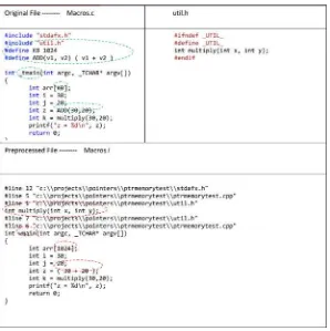
Preprocessing is the process of expanding the macros specified in source files. It also facilitates the conditional compilation and inclusion of header files.
In the code snippet in Figure 1-8 for the file Macros.c, the following are the candidates for preprocessing:
Inclusion of header files
• : util.h, stdafx.h
Whenutil.his included, it includes the declaration of the functionint multiply (int x, int y).
• Expansion of macros: KB, ADD
8
Compilation
The next process is to compile the preprocessed file into assembly code. I will not go into the details of the compilation process, which itself has several phases such as lexical analysis, syntax analysis, code generation, etc. The output of the compilation process is add.asm/add.s. Below is the listing for the add.c program, which is compiled, and its output can be seen in the listing of file add.asm.
File add.c
int add(int v1, int v2) {
return v1+v2; }
int _tmain(int argc, _TCHAR* argv[]) {
int a = 10; int b = 20;
int z = add(10,20); return 0;
}
File add.asm
; COMDAT ?add@@YAHHH@Z _TEXT SEGMENT
_v1$ = 8 ; size = 4 _v2$ = 12 ; size = 4 ?add@@YAHHH@Z PROC ; add, COMDAT ; Line 7
Push ebp Mov ebp, esp
Sub esp, 192 ; 000000c0H Push ebx
Push esi Push edi
Lea edi, DWORD PTR [ebp-192]
Mov ecx, 48 ; 00000030H Mov eax, -858993460 ; ccccccccH rep stosd
; Line 8
Mov eax, DWORD PTR _v1$[ebp] Add eax, DWORD PTR _v2$[ebp] ; Line 9
Pop edi pop esi pop ebx mov esp, ebp pop ebp ret 0
PUBLIC _wmain
EXTRN __RTC_CheckEsp:PROC
; Function compile flags: /Odtp /RTCsu /ZI ; COMDAT _wmain
_TEXT SEGMENT
_z$ = -32 ; size = 4 _b$ = -20 ; size = 4 _a$ = -8 ; size = 4 _argc$ = 8 ; size = 4 _argv$ = 12 ; size = 4 _wmain PROC ; COMDAT ; Line 11
Push ebp mov ebp, esp
sub esp, 228 ; 000000e4H push ebx
push esi push edi
lea edi, DWORD PTR [ebp-228]
mov ecx, 57 ; 00000039H mov eax, -858993460 ; ccccccccH rep stosd
; Line 12
Mov DWORD PTR _a$[ebp], 10 ; 0000000aH ; Line 13
Mov DWORD PTR _b$[ebp], 20 ; 00000014H ; Line 14
Push 20 ; 00000014H push 10 ; 0000000aH call ?add@@YAHHH@Z ; add add esp, 8
mov DWORD PTR _z$[ebp], eax ; Line 15
Xor eax, eax ; Line 16
Pop edi pop esi pop ebx
add esp, 228 ; 000000e4H cmp ebp, esp
10
Assembler
After the compilation process, the assembler is invoked to generate the object code. The assembler is the tool that converts assembly language source code into object code. The assembly code has instruction mnemonics, and the assembler generates the equivalent opcode for these respective mnemonics. Source code may have used external library functions (such as printf(), pow()). The addresses of these external functions are not resolved by the assembler and the address resolution job is left for the next step, linking.
Linking
Linking is the process whereby the linker resolves all the external functions’ addresses and outputs an executable in ELF/COFF or any other format that is understood by the OS. The linker basically takes one or more object files, such as the object code of the source file generated by compiler and also the object code of any library function used in the program (such as printf, math functions from a math library, and string functions from a string library) and generates a single executable file.
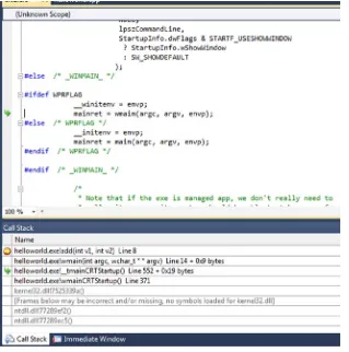
Importantly, it links the startup routine/STUB that actually calls the program’s main routine. The startup routine in the case of Windows is provided by the CRT dll, and in the case of Linux it is provided by glibc (libc-start.c). Figure 1-9 shows what the startup stub looks like.
Figure 1-9. Startup stub
Loader
Strictly speaking, the loader is not part of compilation process. Rather, it is part of the operating system that is responsible for loading executables into the memory. Typically, the major responsibilities of a UNIX loader are the following:
Validation •
Copying the executable from the disk into main memory •
Setting up the stack •
Setting up registers •
Jumping to the program’s entry point (_start) •
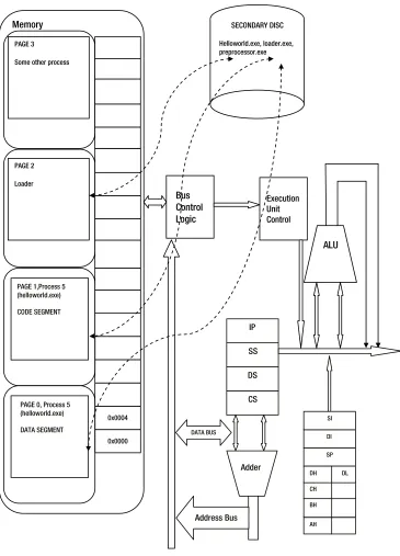
Figure 1-11 depicts a situation in which the loader is executing in memory and loading a program, helloworld. exe. The following are the steps taken by the OS when a loader tries to load an executable:
1. The loader requests that the operating system create a new process.
12
3. It marks the page table with invalid entries.
4. It starts executing the program which generates immediate page fault exception.
SECONDARY DISC
Helloworld.exe, loader.exe, preprocessor.exe
Bus Control Logic
Execution Unit Control
ALU Memory
Address
FRAME 2PAGE 2
Loader
FRAME 3
PAGE 3
Some other process
Adder DATA BUS
Address Bus CS DS SS IP
SP DI SI
AH BH CH DH DL
PAGE 1,Process 5 (helloworld.exe)
CODE SEGMENT
PAGE 0, Process 5 (helloworld.exe)
DATA SEGMENT
0x0004
0x0000
The steps mentioned above are taken care of by the operating system for each program running in the memory. I will not go into the details of the technicalities in these steps; an interested reader can look into operating system-related books for this information.
Let’s see how different programs look when they simultaneously share the physical memory. Let’s assume the operating system has assigned a process id – 5 for the program helloworld.exe. It has allocated FRAME 0 & 1 and loaded the PAGE 0 & 1 where some portion of code segment and data segment are residing currently. We will look at the details of the different segments depicted in Figure 1-11 later in subsequent sections. Page is a unit of virtual memory and Frame is the unit used in the context of physical memory.
Memory Models
A process accesses the memory using the underlying memory models employed by the hardware architecture. Memory models construct the physical memory’s appearance to a process and the way the CPU can access the memory. Intel’s architecture is has facilitated the process with three models to access the physical memory, discussed in turn in the following sections:
Real address mode memory model •
Flat memory model •
Segmented memory model •
Real Address Mode Memory Model
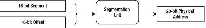
The real address modememory model was used in the Intel 8086 architecture. Intel 8086 was 16 processors, with 16-bit wide data and address buses and an external 20-bit-wide address bus. Owing to the 20-bit-wide address bus, this processor was capable of accessing 0 – (220 – 1) = 1MB of memory; but due owing to the 16-bit-wide address bus, this processor was capable of accessing only [0 – (216 -1)] = 64KB of memory. To cross the 64KB barrier and access the higher address range of 1MB, segmentation was used. The 8086 had four 16-bit segmentation registers. Segmentation is achieved in real mode by shifting 4 bits of a segment register and adding a 16-bit offset to it, which eventually forms a 20-bit physical address. This segmentation scheme was used until the 80386, which had 32-bit-wide registers. This model is still supported to provide compatibility with existing programs written to run on the Intel 8086 processor.
Address Translation in Real Mode
Figure 1-12 depicts how an address translation is done in real mode using segmentation.
16-bit Segment
16-bit Offset
Segmentation
Unit 20-bit Physical Address
14
Flat Memory Model
In the 386 processor and later, apart from the general-purpose 32-bit registers, the designers have provided the following memory management registers to facilitate more sophisticated and complex management:
global descriptor table register (GDTR) •
load descriptor table register (LDTR) •
task register •
In the flat memory model, the memory space appears continuous to the program. This linear address space (i.e., address space accessible to the processor) contains the code segment, data segment, etc. The logical address generated by the program is used to select an entry in the global descriptor table and adds the offset part of the logical address to the segments base, which eventually is equivalent to the actual physical address. The flat memory model provides for the fastest code execution and simplest system configuration. Its performance is better than the 16-bit real-mode or segmented protected mode.
Segmented Memory Model
Unlike segmentation in real mode, segmentation in the segmented memory model is a mechanism whereby the linear address spaces are divided into small parts called segments. Code, data, and stacks are placed in different segments. A process relies on a logical address to access data from any segment. The processor translates the logical address into the linear address and uses the linear address to access the memory. Use of segmented memory helps prevent stack corruption and overwriting of data and instructions by various processes. Well-defined segmentation increases the reliability of the system.
Figure 1-13 gives a pictorial overview of how memory translation takes places and how the addresses are visible to a process.
Memory Layout Using Segments
A multiprogramming environment requires clear segregation of object files into different sections to maintain the multiple processes and physical memory. Physical memory is a limited resource, and with user programs it is also shared with the operating system. To manage the programs executing in memory, they are distributed in different sections and loaded and removed according to the policies implemented in the OS.
To reiterate, when a C program is loaded and executed in memory, it consists of several segments. These segments are created when the program is compiled and an executable is formed. Typically, a programmer or compiler can assign programs/data to different segments. The executable’s header contains information about these segments along with their size, length, offset, etc.
Segmentation
Segmentation is a technique used to achieve the following goals:
Multiprogramming •
Memory protection •
Dynamic relocation •
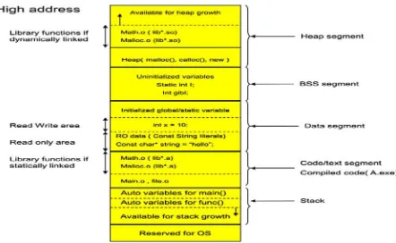
Source code after compilation is segregated into five main sections/segments—CODE, DATA, BSS, STACK, and HEAP—discussed in turn in the following sections.
Code Segment
This segment consists of instruction codes. The code segment is shared among several processes running the same binary. This section usually has read and execute permissions. Statically linked libraries increase the footprints of the executable and eventually the code segment size. They execute faster than dynamically-linked libraries.
Dynamically-linked libraries reduce the footprint of the executable and eventually the code segments’ size. They execute more slowly because they spend time in loading the desired library during runtime.
Main.c foo.c void main() void foo() { {
foo(); return; return;
} }
All the generated machine instructions of the above code from Main.c and foo.c will be part of a code segment.
Data Segment
A data segment contains variables that are global and initialized with nonzero values, as well as variables that are statically allocated and initialized with nonzero values. A private copy of the data segment is maintained by each process running the same program.
A static variable can be initialized with a desired values before a program starts, but it occupies memory
16
Source code Main.c
static int staticglobal = 1; int initglobal = 10;
int uninitglobal; void main() {
return; }
The variables staticglobal and initglobal are part of the data segment.
Uninitialized/BSS Segment
BSS stands for “Block Started by Symbol.” It includes all uninitialized global variables as well as uninitialized static local variables declared with the static keyword. All the variables in this section are initialized to zero by default. Each process running the same program has its own data segment. The size that BSS will require at runtime is recorded in an object file. BSS does not take up any actual space in an object file. Initialization of this section is done during startup of the process. Any variable that requires initialization during startup of a program can be kept here when that is advantageous. The following source code illustrates an example where the variables declared are part of a BSS segment.
Source code Main.c
static int uninitstaticglbl; int uninitglobal;
void main() {
return; }
The variables uninitstaticglbl and uninitglobal are part of BSS segment.
Stack Segment
The stack segment is used to store local variables, function parameters, and the return address. (A return address is the memory address where a CPU will continue its execution after the return from a function call).
Local variables are declared inside the opening left curly brace of a function body, including the main() or other left curly braces that are not defined as static. Thus, the scopes of those variables are limited to the function’s body.
The life of a local variable is defined until the execution control is within the respective function body.
main.c foo.c void main() void foo() { {
int var1; int var3; int var2 = 10; int var4; foo();
} }
Heap Segment
The heap area is allocated to each process by the OS when the process is created. Dynamic memory is obtained from the heap. They are obtained with the help of the malloc(), calloc(), and realloc() function calls. Memory from the heap can only be accessed via pointers. Process address space grows and shrinks at runtime as memory gets allocated and deallocated. Memory is given back to the heap using free(). Data structures such as linked lists and trees can be easily implemented using heap memory. Keeping track of heap memory is an overhead. If not utilized properly, it may lead to memory leaks.
Runtime Memory Organization
The runtime memory organization can be viewed In its entirety in the Figure 1-14. You can see that some portions of memory are used by the operating system and rest are used by different processes. The different segments of a single process and different segments belonging to other processes are both present during runtime.
Figure 1-14. Runtime memory organization
Intricacies of a Function Call
18
The allocated stack frame is used to store the automatic variables, parameters, and return address. Recursive or nested calls to the same function will create separate stack frames. The size of the stack frame is a limited resource which needs to be considered while programming.
Maintenance of the stack frame and the entities included inside it (local variables, return address, etc.) is achieved with the help of following registers:
• base pointer/frame pointer (EBP): Used to reference local variables and function parameters in the current stack frame.
• stack pointer (ESP): Always points to the last element used on the stack.
• instruction pointer (EIP): Holds the address of the next CPU instruction to be executed, and it is saved onto the stack as part of the CALL instruction.
Steps to Make a Function Call
Let’s examine how a function call is made and the various steps involved during the process.
1. Push parameters onto the stack, from right to left.
0x200000000 main() 0x200000004 {
0x200000084 int x = 10; 0x200000089 int y = 20; 0x200000100 int z;
0x200000104 z = add( 10, 20); < --- CALL INSTR [ param #2 (20) ]
0x200000108 z++; < --- EIP [ param #1 (10) ]
0x200000110 }
2. Call the function.
The processor pushes the EIP onto the stack. At this point, the EIP would be pointing to the first byte after the CALL instruction.
3. Save and update the EBP.
At this point we are in the new function. •
Save the current EBP (which belongs to the callee function). •
Push the EBP. •
Make the EBP point to the top of the stack: •
mov ebp, esp
…….
param #2 ( 20)
param #1 (10)
Layout of stack at this point
…….
param #2 ( 20)
param #1 (10)
EBP can now access the function parameters as follows:
8(%ebp) – To access the 1st parameter.
12(%ebp) – To access the 2nd parameter.
And so on…
The above assembly code is generated by the compiler for each function call in the source code.
Save the CPU registers used for temporaries. •
Allocate the local variables. •
int add( int x, int y) {
int z; z = x + y; return z; }
The local variable is accessed as follows: -4( %ebp ), -8( %ebp ) etc..
Layout of stack at this point
< --- current EBP
…….
param #2 ( 20)
param #1 (10)
20
4. Returning from the function call. Release local storage.
•
By using a series of POP instructions •
Restore the saved registers •
Restore the old base pointer •
Return from the function by using the RET instruction •
Considering the temporal and spatial locality behavior exhibited by programs while executing, the stack segment is the optimum place to store data, because many programming constructs—such as for loop and do while—tend to reuse the same memory locations. Making a function call is an expensive operation as it involves a time-consuming setup of the stack frame. Inline functions are preferred instead when the function body is small.
Memory Segments
In the previous sections, you saw various segments involved during the runtime of an application. The following source code helps in visualizing and analyzing the formation of these segments during runtime. The program is self-explanatory. It prints the addresses of all the segments and the address of variables residing in their respective segments.
Source code Test.c
#include<stdio.h> #include<malloc.h>
int glb_uninit; /* Part of BSS Segment -- global uninitialized variable, at runtime it is initialized to zero */
Layout of stack at this point
< --- return address < --- current EBP
< --- current ESP
…….
param #2 ( 20)
param #1 (10)
OLD EBP OLD EIP 0x200000108
Local var #1 ( z )
Saved %reg
int glb_init = 10; /* Part of DATA Segment -- global initialized variable */ void foo(void)
{
static int num = 0; /* stack frame count */
int autovar; /* automatic variable/Local variable */ int *ptr_foo = (int*)malloc(sizeof(int));
if (++num == 4) /* Creating four stack frames */ return;
printf("Stack frame number %d: address of autovar: %p\n", num, & autovar); printf("Address of heap allocated inside foo() %p\n",ptr_foo);
foo(); /* function call */ }
int main() {
char *p, *b, *nb;
int *ptr_main = (int*)malloc(sizeof(int)); printf("Text Segment:\n");
printf("Address of main: %p\n", main); printf("Address of afunc: %p\n",foo); printf("Stack Locations:\n");
foo();
printf("Data Segment:\n");
printf("Address of glb_init: %p\n", & glb_init); printf("BSS Segment:\n");
printf("Address of glb_uninit: %p\n", & glb_uninit); printf("Heap Segment:\n");
printf("Address of heap allocated inside main() %p\n",ptr_main); return 0;
}
Output:
Text Segment:
Address of main: 00411131 Address of afunc: 004111CC Stack Locations:
Stack frame number 1: address of autovar: 0012FE5C Address of heap allocated inside foo() 003A2E78 Stack frame number 2: address of autovar: 0012FD70 Address of heap allocated inside foo() 003A2EB8 Stack frame number 3: address of autovar: 0012FC84 Address of heap allocated inside foo() 003A2EF8 Data Segment:
Address of glb_init: 00417014 BSS Segment:
Address of glb_uninit: 00417160 Heap Segment:
22
Virtual Memory Organization
Multiprogramming enables many processes to execute concurrently at any given time. It is not necessary that these processes be interrelated. The support is enabled by hardware (the memory management unit) and the operating system. Virtual memory allows the operating system to use system resources optimally. The most important feature of virtual memory organization is the protection of various processes from one another by the operating system.
The features of virtual memory include the following:
Physical organization •
Logical organization •
Protection •
Relocation •
Sharing •
In a multiprogramming environment, many processes share the main memory. A process as a whole sees the main memory as a complete resource dedicated to itself (the process). But the operating system loads/keeps only that portion of a program in memory that is currently required to be executed.
A Glimpse into a Virtual Memory System
Figure 1-15 illustrates how a virtual address space is mapped to a physical address. The main entities that take part in this translation are MMU, TLB, and page tables, described in the next section.
Physical Memory CPU
MMU
TLB
Virtual Address
Page Tables
Physical Address
Figure 1-15. Virtual memory system
Address Spaces
Memory space has to be shared between two entities:
The kernel/OS •
By definition any program, whether an OS or a user program, is termed a kernel process or a user process when loaded in memory.
Virtual Address Space
Virtual memory is a logical entity whereby a user process assumes that it is loaded. The address pertaining to this virtual memory is called the virtual address space.
Figure 1-16 shows a typical scenario whereby a process assumes it is loaded. The virtual address space from 0 - 7FFFFFFE is being used to load the user process. The virtual address 0x7FFFFFFF – higher is used by the kernel. When a program is loaded into memory, the respective process assumes that the whole user space is allocated for the process.
Kernel Memory
Process List
0xffffffff
Kernel Stack
OX7fffffff
Stack
0x00000000 Text
0xffffffff
Kernel Stack
OX7fffffff
Stack
0x00000000 Text
0xffffffff
Kernel Stack
OX7fffffff
Stack
0x00000000 Text
Figure 1-17. Kernel’s view of virtual address space
Figure 1-16. Process’s view of virtual address space
24
A virtual address consists of
A virtual page number •
A page offset field •
Physical Address Space
The physical address space is the actual address in the main memory where the pages are loaded. Figure 1-18 illustrates a typical scenario of how a virtual address is translated into a physical address.
Virtual Page Number Page Offset
31 11 0
Paging
Paging is one of the most important parts of virtual memory. This scheme allows the operating system to load and unload the parts of pages of a process to any non-contiguous location of physical memory. The notion of paging assumes that the main/physical memory is divided into equal and fixed size frames/page frames which can accommodate pages of any process. Pages are basically parts of processes that are divided into equal and fixed size, typically 1kb/4kb.
Figure 1-19 illustrates a paging scenario where pages of process A and process B are residing in various frames of physical memory.
Virtual Page Number Page Offset
31 11 0
Physical Page Number Page Offset
31 11 0 Address Translation
Frame 0 Frame 1 Frame 2 Frame 3 Frame 4 Frame 5
Physical memory
PAGE 0 PAGE 1 PAGE 2 PAGE 3 PAGE 4 PAGE 5 PAGE 0
PAGE 1 PAGE 2 PAGE 3 PAGE 4 PAGE 5
Process B’s VM Process A’s VM
Figure 1-19. Paging
The paging system typically addresses the following tasks:
1. Address Space Management: Responsible for allocating and managing the address space of processes
2. Address Translation: Done by dedicated hardware in the MMU. It also takes care of exception handling (such as page faults)
3. Memory Sharing: This is shown in Figure 1-19.
Page Table
26
Summary
This chapter has discussed relevant aspects of memory—in particular, memory classification and cache memory. Aspects of cache memory that I have not discussed, such as performance optimization and the CPU generating exceptions due to alignment issues, are not required in the current context. The most important section of this chapter is the one on memory layout, which serves to strengthen the knowledge of the reader from a programming as well as from a systems point of view.
The next chapter develops the basics of pointer variable concepts and other details such as memory allocation and its usage.
Physical Memory
SWAP DISK Virtual Page
Page Table
VALID
0
1
1
1
0
0
0
1
1
Pointer Basics
Like any other variable, you need to first understand the basics of pointer variables. The basics include declaration, definition, and usage. This chapter explains the concept of pointer variables. The emphasis is on the usage of pointers with the help of diagrams to visualize the concepts. This chapter also explains the inner details of memory allocation and deallocation, and how pointer variables manipulate them.
Pointers by definition are variables used to store memory addresses of data or functions, unlike other data type variables that are used to store only the value. As with any usual variable, a pointer takes space in memory. In the next section, we will concentrate first on the concept of referencing/dereferencing of variables, as it will help visualize how a pointer works.
What is an address of a variable?
Consider the following:int x = 40;
0x00394768 ----> x = 40
The drawing above shows how a variable x of type integer is used to store the value of 40. For a program, the variable x is nothing but a storage location of some memory address. In the above case, we are storing the value of 40 at location 0x00394768, and this location is referred to by the variable x. This also means that any variable we have used in our program refers to some address. If you remember from Chapter 1, there are code segments for each program. The functions also share that part of the memory, and they are loaded at some other part of the code segment itself.
In the above case, we are trying to store an integer value, but notice that a memory address is also a number or value. What if we want to store that number in some other variable? If we want to store or access a memory address (such as 0x00394768) in a variable, we need special variables called pointers.
Address of Operator
28
Source code. Ptr1.c
int main() {
int var_int ;
printf("Insert data\n"); scanf("%d", &var_int); return 0;
}
In the example above, the function scanf uses the “address of” operator (&) to get the address of the variable var_int to store the value entered by the user, because the scanf function should know the address where the value needs to be kept.
Retrieving the Address of a Variable
As mentioned earlier, data is stored in a memory location. The following program illustrates how to obtain the address of the memory location or the address of the variable where data is stored.
Source code. Ptr2.c
int main() {
int var_int = 40;
printf ("Address of variable \"var_int\": %p\n", &var_int); }
Output:
Address of variable "var_int": 00394768
In the example above, we used the & operator to get the address of the variable.
If we extend the concept of address to a structure variable, where the structure variable itself contains many other variables, we can retrieve their addresses with the help of the “address of” operator.
Source code Ptr3.c
struct node{ int a; int b; };
int main() {
struct node p;
printf("Address of node = %p\n",&p);
printf("Address of member variable a = %p\n", &(p.a)); printf("Address of member variable b = %p\n", &(p.b)); return 0;
Output:
Address of node = 003AFB00
Address of member variable a = 003AFB00 Address of member variable b = 003AFB04
Notice in the output above that the address of the first member and the second member in the data structures are very nearby. This means that for any number of member fields inside a structure, the addresses are allocated sequentially or nearby as per their sizes.
Pointer Declaration
Now you know how an address can be retrieved via the “address of” operator. Next, let’s get a variable to store this address. This particular variable, which is capable of storing and operating on addresses of variables, is called a pointer variable. We will start with the declaration of the pointer variables. Below is the generic form through which we declare the pointer variables:
Datatype* variable_name;
Example 1: A pointer variable capable of pointing and storing addresses of primitive data types.
int* intptr, char* charptr
The declaration of pointer variables involves a special operator called a dereference operator (*) which helps the compiler identify that it is a pointer variable. An associated data type informs the compiler about the kind of variable’s data type address it holds. Both dereference and “address of” operators are unary in nature.
Example 2: Declaring pointers to aggregate data types (structures)
struct inner_node { int in_a; int in_b; };
struct node{ int *a; int *b;
struct inner_node* in_node; };
In the example above, struct inner_node* in_node is a pointer variable, where struct inner_node is a data type and the pointer variable’s name is in_node. As seen above, we can have pointer variables as data members of structures.
Pointer Assignment
30
Making a pointer variable point to a particular memory address can be done in two ways.
1. By assigning the variable’s address with the help of an address of pointers (&).
int x = 40; int *ptr;
ptr = &x; // address of operator used to collect the address of variable x
0x00394768 ---->
0x0012FF60 ---->
x = 40
ptr = 0x00394768
2. By making the pointer variable point to a dynamically allocated memory from the heap.
int * ptr;
ptr = ( int *) malloc(sizeof(int) * count );
0x00394768 ---->
0x0012FF60 ---->
Memory from heap
ptr = 0x00394768
In Case 1, the memory to store a value of 40 in variable x will be allocated during runtime, depending on the scope of the variable. Recall the memory layout sections in Chapter 1.
In Case 2, the memory to store a value is created explicitly using the malloc call, which returns memory from the heap area.
The programmer should keep in mind that any operation on a pointer variable should be done only if it is pointing to a valid memory address; otherwise this will result in a segmentation fault. If the segmentation fault occurs, it will lead the program to crash and eventually it will be stopped.
Size of Pointer Variables
The size of a variable is another important and critical aspect for a programmer. He should know how much a variable consumes when it is used. The size of any pointer variable can be 32-bit or 64-bit, depending on the platform. If a platform is 32-bit, the size of pointer variables (int *, char *, float *, and void *) will be 4 bytes. In fact, pointer variables that store the “address of” aggregate data types, such as arrays and structures, are also of size 4 bytes. Clearly, the memory address size of a pointer variable is 32 bits long.
Source code. Ptr4.c
#include <stdio.h> #include <conio.h> int main()
{
char c_var; int i_var; double d_var; char *char_ptr; int *int_ptr; double *double_ptr; char_ptr = &c_var; int_ptr = &i_var; double_ptr = &d_var;
printf("Size of char pointer = %d value = %u\n", sizeof(char_ptr), char_ptr); printf("Size of integer pointer = %d value = %u\n", sizeof(int_ptr), int_ptr); printf("Size of double pointer = %d value = %u\n", sizeof(double_ptr),double_ptr); getch();
}
Output:
Size of char pointer = 4 value = 4061659 Size of integer pointer = 4 value = 4061644 Size of double pointer = 4 value = 4061628
It is interesting to verify the size consumed by a pointer variable that is pointing to structure variables. The following code illustrates this.
Source code. Ptr5.c
#include <stdio.h> #include <conio.h> struct inner_node {
int in_a; int in_b; };
struct node{ int *a; int *b;
struct inner_node* in_node; };
int main() {
32
printf("Size of pointer variable (struct node*) = %d\n",sizeof(struct node*)); printf("Size of pointer variable pointing to int array = %d\n", sizeof(arrptr)); return 0;
}
Output:
Size of pointer variable (struct node*) = 4 Size of pointer variable pointing to int array = 4
In the example above, the size of the data type struct node* is 4 bytes and conforms to the fact that the size of a memory address is always 4 bytes.
Pointer Dereferencing
Now that you can store and retrieve the address of a variable and store it to a pointer variable successfully, let’s think about what you can do with this achievement. The pointer variable stores the address; to access the value stored at that address you use the “value at” operator (* to be precise). This particular technique is called pointer dereferencing. This is also called indirection in some texts. You will see the advantages of using pointer variables in the coming sections.
Every variable is used to store a value, and this rule is also applicable for pointer variables. The value of a pointer variable is the address of some memory location. Once we store a memory address in a pointer variable, we should be able to find the value stored at this location. Let’s see how this is done with pointer dereferencing.
We need to use the dereferencing operator (*) to get the value stored at some memory location. This operator is also called “value at” operator. Consider the following code:
int x = 10; /* value 10 stored at some memory location */
int *ptr = &x; /* now pointer variable "ptr" is pointing to the memory location x = 10 */ printf("Address of variable \"x\" = %p\n", &x); /* prints the address of memory location x */ printf("Address of variable \"x\" = %p\n", ptr); /*prints the address of memory location x with the help of "ptr" variable, whose value is memory location "x" */
printf("Value of variable \"x\" = %d\n", x); /* prints the value of variable x */
printf("Value stored at address ptr = %p is %d\n", ptr, *ptr); /* prints the value at memory location of x with the help of value at operator (*ptr) */
Essentially the value of variable ptr and the value of the expression (&x) evaluates to one thing: a memory location of variable x, since ptr is pointing to x right now.
To get the value stored at some memory location, we use the dereferencing operator (*). Therefore, the expressions *ptr, *(&x), and x will evaluate to one and the same thing: 10.
Tip
In the first line of Example B, we are trying to keep the value 10 at a location that is not valid since the variable ptr is not pointing to a valid memory location.
To make this program work correctly we need to make the ptr variable point to a valid memory location. The following code illustrates the appropriate method to do this:
int count = 1; //"count" variable will be used to allocate one memory location of size integer type int *ptr = (int *) malloc ( sizeof(int) * count );
Now the ptr variable points to a valid memory location.
*ptr = 10; //At this point we are assigning a value to the memory location where "ptr" is pointing to free(ptr) ; // At this point we freed the memory pointed to by the variable "ptr"
*ptr = 20; // Again at this point the program will throw a segmentation error, because we are trying to access a memory which has already been freed.
Basic Usage of Pointer
You have seen how pointers are declared and initialized. We will now look into the most basic usage of pointers, or rather the advantage of using pointers. Functions and parameters go hand in hand. With pointer variables we have a lot of luxury to manipulate any memory value with the help of indirection. To understand this section, it would be a good idea to refresh the lifecycle, scope of the variable, and stack segment from Chapter 1.
Pass by Value
Functions are capable of receiving information from the caller and returning results back to the caller. This technique is the most basic form of information passing among functions.
y = 10 0x21436587
ptr dereferenced appropriately as it points to a valid address
ptr = junk value
X = 10 0x12345678
Ptr = 0x123456 78 0x87654321
int x = 10;
int *ptr = &x;
int y = *ptr;
Example B Example A
int *ptr = 10;
int y = *ptr; // At this point the program will crash, as we are trying to access a memory location which is not valid
34
Function Signature
int function_name( int param1, int param2, int param3 ... ..);
In the declaration of the function above, the parameters int param1, int param2, and int param3 are called input parameters. The return type of this function declaration is int, which tells that this function will return a value of type integer to the caller function.
In this particular technique, only the values are being passed to the called function. After the values are passed, these values are copied onto the respective stack of the called function. Similarly, the exact process is repeated for the returned value of the called function.
void calling_function(void) {
int t1, t2, t3; t1 = 10; t2 = 20;
t3 = called_function(t1, t2); }
int called_function(int x, int y) {
int t1, t2, t3; t1 = x;
t2 = y; t3 = t1 + t2; return t3; }
Pass by Reference
This is another technique of passing information among functions. Pass by reference is used to pass the memory address of variables rather than the value itself.
Function Signature
int* function_name( int* param);
In the function declaration above, the input parameter param is of int*, which is expecting to receive the address of an integer variable from the calling function. And this function will also be returning the address of an integer variable to the calling function.
t1 = 10
t2 = 20
t3 = 30
Local copy of the calling_function
t1 = 10
t2 = 20
t3 = 30
void calling_function(void) {
int t1; int *t2; t1 = 10;
t2 = called_function(&t1); }
int* called_function(int* x) {
int t2; int *t1; int *t3; t1 = x; t2 = 10;
t3 = (int*)malloc(sizeof(int)); t3 = *t1 + t2;
return &t3; }
In the case above, only the address of a variable is passed to the called function, which then is copied to the stack. This technique has two advantages as compared to the former technique.
1. Amount of data being copied: Although the copying of the parameter is carried out in this case as well (i.e., the copying of the memory address), the amount of information that is copied will always be 4 bytes. In the example above, the amount (size) of information that is passed is the same.
Case 1: Pass by value
struct data {
int x; int y; };
void func(struct data v1) {
struct data v2 = v1; }
int main() {
struct data var; var.x = 10; var.y = 20; func( var ); return 0; }
In the example above, the size of the variable struct data is 8 bytes. Since pass by value is used, 8 bytes are copied onto the stack of the called function func.
t1 = 0X12345678
t2 = 20
Local copy of called_function t1 = 10 ---0X12345678
t2 = 0X87654321
36
Case 2: Pass by reference
struct data {
int x; int y; };
void func(struct data* v1) {
struct data *v2 = v1; }
int main() {
struct data var; var->x = 10; var->y = 20; func(& var ); return 0; }
In the example above, the size of the parameter is 4 bytes since we passed the pointer to the structure variable.
2. Accessibility of variables: The pass by reference technique makes it possible to manipulate the local variables of a function from a different function.
Pointers and Constants
You may have heard of the keyword const and used it in programming. A normal variable use of const has one meaning. The value assigned during initialization will never change throughout the lifetime of the variable in its scope. However, the use of the pointers and constants together can have a varied affect.
Constant Pointer Variable
A constant pointer is a pointer variable that is meant to point to only one memory address. Therefore, the value of the pointer variable cannot be changed.
Declaration of constant pointer: <pointer type*> const <variable name> Example: int* const ptr1, char* const ptr2;
Here are the rules for using constant pointers.
1. Constant pointer variables must be initialized during declaration.
Source code. Ptr6.c
int main() {
int num = 10;
2. Once initialized, the const pointer should not point to any other memory address.
Source code. Ptr7.c
#1. int main() #2. {
#3. int num1 = 10; #4. int num2 = 20;
#5. int* const ptr1 = &num1; //Initialization of const ptr
#6. ptr1 = &num2; // can’t do this
#7. printf("Value stored at pointer = %d\n",*ptr1); #8. }
In the program above, the constant pointer variable ptr1 is initialized at line #5 and is pointing to the memory address of the variable int num1. At line #6, the program is trying to make the constant pointer variable ptr1 point to the memory address of the variable int num2. When this particular piece of code is compiled, the compiler will throw a compilation error.
Pointer to Constant Variable
A pointer to a constant variable is a concept where the value of a pointer variable (i.e., a memory address of a non-constant variable) should not modify the value at that particular memory address. Different pointers could point to that specific variable.
Declaration of constant pointer: const<pointer type*> <variable name> Example: const int* ptr1, const char* ptr2;
0x123456 num1 = 10
0x654321 num2 = 20
0x111122 Const Ptr1 = 0x123456 Mem addr values
0x123456 num1 = 10
0x654321 num2 = 20
38
Source code. Ptr8.c
#1. int main() #2. {
#3. int num1 = 10; #4. const int* ptr1;
#5. int* ptr2; #6. ptr1 = &num1;
#7. *ptr1 = 20; //can’t do this #8. num1 = 20; //can be done
#9. printf("Value stored at pointer = %d\n",*ptr1); #10. }
When we try to compile the code above, the compiler will throw a compilation error because of line #7.
Constant Pointer to a Constant Variable
A constant pointer to a constant variable is a concept where a pointer variable is constant; in other words, the pointer variable will only point to a memory address where it is initialized, and later the pointer should not point to any other memory location. Additionally, the value stored at that particular address should not be modified by that particular pointer. In summary, we cannot change the value of a pointer variable and we cannot modify the value stored at that address.
Declaration of constant pointer: const<pointer type*> const <variable name> Example: const int*const ptr1, const char* const ptr2;
Source code. Ptr9.c
#1. int main() #2. {
#3. int num1 = 10; #4. int num2 = 20;
#5. const int* ptr1 = &num1; #6. int* ptr2;
#7. *ptr1 = 20; //cannot change the value that the const pointer is pointing to #8. num1 = 20; //can be done
#9. ptr1 = &num2; //cannot change the constant pointer’s value (i.e. – constant pointer should //not point to any other memory address once initialized
#10.printf("Value stored at pointer = %d\n",*ptr1); #11. }
When we try to compile the code above, the compiler will throw a compilation error because of line #7 and line #9.
0x123456 num1 = 10
0x111122 ptr1 = 0x123456 Mem addr values
0x123456 num1 = 20
Multilevel Pointers
Until now, you have seen and worked with one level of indirection. You may have thought about the possibility of multilevel indirection. As you saw earlier, pointer variables are able to store the memory address of other variables, and it is possible to extend this notion further. The address of a pointer variable itself can be stored in any other pointer variable.
The variable used for storing an address of a pointer variable is called a pointer to pointer variable. We can extend this more, such as pointer to pointer to pointer variable and so forth.
Pointer to a Pointer Variable
We will now discuss the second level of pointer indirection. Consider the following piece of code:
int a = 10; int *ptr = &a;
In this code, we have declared an integer variable a and an integer pointer variable ptr, which is pointing to that integer variable. Now we will see how to store the address of this integer pointer variable into another pointer variable. To be able to store the address of a pointer variable into another variable, we need a different kind of variable.
Declaration: <data type >** <variable_name>
The number of asterisks depends on the level of indirection. We keep on increasing the number of asterisks as the level of indirection increases.
int a = 10; int *ptr = &a; int **ptr1 = &ptr;
Source code. Ptr10.c
int main() {
int num = 10; int *ptr = # int **mptr = &ptr;
printf("Value of var num = %d\n", num); printf("Value of var num = %d\n", *ptr); printf("Value of var num = %d\n", **mptr);
printf("Address of var num = %p\n", &num); printf("Address of var num = %p\n", ptr); printf("Address of var num = %p\n", *mptr);
printf("Address of pointer var ptr = %p\n",&ptr); printf("Address of pointer var ptr = %p\n",mptr); printf("Address of pointer var mptr = %p\n",&mptr);
return 0; }
0x123456 a = 10
0x111122 ptr = 0x123456 Mem addr values
40
Understanding a Cryptic Pointer Expression
Understanding pointer expressions becomes cryptic due to the many ways a pointer address can be dereferenced. In this section, we will focus on segregating the equivalent expressions and thus understanding these expressions more easily. You may find this section iterative, but it is a good idea to collate all of the information together.
We will begin by considering the case of one level of indirection. In all further discussions, we will consider an integer variable with its value initialized to 10 and its storage at memory location 0x0001. We will see equivalence of these expressions with two scenarios (referencing and dereferencing).
Referencing
int val = 10;Varname/Addr Value
val/0x0001 10
int *ptrvar = &val;
Varname/Addr Value Varname/Addr Value
val/0x0001 10
ptrvar/0x0005 0x0001
Since the pointer variable ptrvar is storing the address of the variable val, and the expression &val yields the same value, both of these expressions are equivalent. Therefore, we can say ptrvar == &val.
Dereferencing
As you know, to dereference we use the “value at” (*) operator. If we try to use this operator on a pointer variable, it will yield the value stored at the memory address that is stored in that location.
Varname/Addr Value Varname/Addr Value val/0x0001 10 ptrvar/0x0005 0x0001
Value at ( *)
*ptrvar == 10
Also, in the section referenced above, we saw that ptrvar == &val. We can use the “address of” operator expression to yield the same value.
*(&val) == 10
Now, let’s do the same exercise with two levels of indirection. We will use the same two variables that we used above, and a new variable to store the address of an integer pointer variable.
a. int val = 10;
b. int *ptrvar = &val;
c. int **ptrptrvar = &ptrvar; Let’s start with referencing.
Referencing
For the first two variables, the schematic memory diagram will be the same as what we drew earlier in the one level indirection case. For the third variable that is a pointer to a pointer variable of type integer, refer to the following schematic diagram.
int **ptrptrvar = &ptrvar;
Varname/Addr Value Varname/Addr Value Varname/Addr Value val/0x0001 10 ptrvar/0x0005 0x0001
ptrptrvar/0x0009 0x0005
The variable ptrptrvar is a pointer to pointer variable that is storing the address of a pointer variable. Therefore, we verify the expression ptrptrvar == &ptrvar.
Dereferencing
In this section, we will apply the value at operator to the top most level and then we will see how the meanings of the expressions change.
*ptrptrvar == ptrvar == 0x0001
Since ptrptrvar == &ptrvar, we can obtain the same value by another equivalent expression.
*(&ptrvar) == 0x0001
Therefore, *ptrptrvar == ptrvar == *(&ptrvar) == 0x0001.
Now, we will apply the second level of indirection: **ptrptrvar, this expression will yield the value 10. We can write **ptrptrvar == 10.
In the expression above, if we try to replace the *ptrptrvar part, we can substitute its equivalent expression mentioned above to get the same result. Therefore, **ptrptrvar == *(ptrvar) == *(*(&ptrvar) ) == 10.
The same concept that we discussed above is explained with the help of Figure 2-1.
42
Summary
In this chapter we covered the basics of pointers and their usage. The goal of this chapter is that you understand the concept of referencing and dereferencing. You should concentrate more on this concept with multilevel indirections. Pointers with structure variables are covered in very minimalist form in this chapter; an upcoming chapter is dedicated solely to understanding pointers when they are used for structure type variables.
In the next chapter, we will look into more advanced concepts of pointer arithmetic. We will also cover the use o