Optimizing Java
Optimizing Java
by Benjamin J Evans and James Gough
Copyright © 2016 Benjamin Evans, James Gough. All rights reserved. Printed in the United States of America.
Published by O’Reilly Media, Inc., 1005 Gravenstein Highway North, Sebastopol, CA 95472.
O’Reilly books may be purchased for educational, business, or sales promotional use. Online editions are also available for most titles (http://safaribooksonline.com). For more information, contact our corporate/institutional sales department: 800-998-9938 or
Editors: Brian Foster and Nan Barber
Revision History for the First Edition
2016-MM-YY First Release
See http://oreilly.com/catalog/errata.csp?isbn=0636920042983 for release details.
The O’Reilly logo is a registered trademark of O’Reilly Media, Inc.
Optimizing Java, the cover image, and related trade dress are trademarks of O’Reilly Media, Inc.
While the publisher and the authors have used good faith efforts to ensure that the information and instructions contained in this work are accurate, the publisher and the authors disclaim all responsibility for errors or omissions, including without limitation responsibility for damages resulting from the use of or reliance on this work. Use of the information and instructions contained in this work is at your own risk. If any code samples or other technology this work contains or describes is subject to open source licenses or the
intellectual property rights of others, it is your responsibility to ensure that your use thereof complies with such licenses and/or rights.
Preface
Chapter 1. Optimization and
Performance Defined
Optimizing the performance of Java (or any other sort of code) is often seen as a Dark Art. There’s a mystique about performance analysis - it’s often seen as a craft practiced by the “lone hacker, who is tortured and deep thinking” (one of Hollywood’s favourite tropes about computers and the people who operate them). The image is one of a single individual who can see deeply into a system and come up with a magic solution that makes the system work faster.
This image is often coupled with the unfortunate (but all-too common)
situation where performance is a second-class concern of the software teams. This sets up a scenario where analysis is only done once the system is already in trouble, and so needs a performance “hero” to save it. The reality,
Java Performance - The Wrong Way
For many years, one of the top 3 hits on Google for “Java Performance Tuning” was an article from 1997-8, which had been ingested into the index very early in Googles history. The page had presumably stayed close to the top because its initial ranking served to actively drive traffic to it, creating a feedback loop.
The page housed advice that was completely out of date, no longer true, and in many cases detrimental to applications. However, the favoured position in the search engine results caused many, many developers to be exposed to terrible advice. There’s no way of knowing how much damage was done to the performance of applications that were subjected to the bad advice, but it neatly demonstrates the dangers of not using a quantitative and verifiable approach to performance. It also provides another excellent example of not believing everything you read on the Internet.
NOTE
The execution speed of Java code is highly dynamic and fundamentally depends on the underlying Java Virtual Machine (JVM). The same piece of Java code may well execute faster on a more recent JVM, even without recompiling the Java source code.
As you might imagine, for this reason (and others we’ll discuss later) this book does not consist of a cookbook of performance tips to apply to your code. Instead, we focus on a range of aspects that come together to produce good performance engineering:
Performance methodology within the overall software lifecycle
Theory of testing as applied to performance
Measurement, statistics and tooling
Underlying technology and mechanisms
Later in the book, we will introduce some heuristics and code-level
techniques for optimization, but these all come with caveats and tradeoffs that the developer should be aware of before using them.
NOTE
Please do not skip ahead to those sections and start applying the techniques detailed without properly understanding the context in which the advice is given. All of these techniques are more than capable of doing more harm than good without a proper understanding of how they should be applied.
In general, there are no:
Magic “go-faster” switches for the JVM
“Tips and tricks”
Secret algorithms that have been hidden from the uninitiated
Performance as an Experimental Science
Performance tuning is a synthesis between technology, methodology,
measurable quantities and tools. Its aim is to affect measurable outputs in a manner desired by the owners or users of a system. In other words,
performance is an experimental science - it achieves a desired result by: Defining the desired outcome
Measuring the existing system
Determining what is to be done to achieve the requirement
Undertaking an improvement exercise to implement
Retesting
Determining whether the goal has been achieved
The process of defining and determining desired performance outcomes builds a set of quantative objectives. It is important to establish what should be measured and record the objectives, which then forms part of the project artefacts and deliverables. From this, we can see that performance analysis is based upon defining, and then achieving non-functional requirements.
This process is, as has been previewed, not one of reading chicken entrails or other divination method. Instead, this relies upon the so-called dismal
methods of statistics. In Chapter 5 we will introduce a primer on the basic statistical techniques that are required for accurate handling of data generated from a JVM performance analysis project.
A Taxonomy for Performance
In this section, we introduce some basic performance metrics. These provide a vocabulary for performance analysis and allow us to frame the objectives of a tuning project in quantitative terms. These objectives are the non-functional requirements that define our performance goals. One common basic set of performance metrics is:
Throughput
Throughput is a metric that represents the rate of work a system or subsystem can perform. This is usually expressed as number of units of work in some time period. For example, we might be interested in how many transactions per second a system can execute.
For the throughput number to be meaningful in a real performance exercise, it should include a description of the reference platform it was obtained on. For example, the hardware spec, OS and software stack are all relevant to
Latency
Performance metrics are sometimes explained via metaphors that evokes plumbing. If a water pipe can produce 100l per second, then the volume produced in 1 second (100 litres) is the throughput. In this metaphor, the latency is effectively the length of the pipe. That is, it’s the time taken to process a single transaction.
Capacity
The capacity is the amount of work parallelism a system possesses. That is, the number units of work (e.g. transactions) that can be simultaneously ongoing in the system.
Capacity is obviously related to throughput, and we should expect that as the concurrent load on a system increases, that throughput (and latency) will be affected. For this reason, capacity is usually quoted as the processing
Utilisation
One of the most common performance analysis tasks is to achieve efficient use of a systems resources. Ideally, CPUs should be used for handling units of work, rather than being idle (or spending time handling OS or other housekeeping tasks).
Depending on the workload, there can be a huge difference between the
Efficiency
Dividing the throughput of a system by the utilised resources gives a measure of the overall efficiency of the system. Intuitively, this makes sense, as
requiring more resources to produce the same throughput, is one useful definition of being less efficient.
Scalability
The throughout or capacity of a system depends upon the resources available for processing. The change in throughput as resources are added is one
measure of the scalability of a system or application. The holy grail of system scalability is to have throughput change exactly in step with resources.
Consider a system based on a cluster of servers. If the cluster is expanded, for example, by doubling in size, then what throughput can be achieved? If the new cluster can handle twice the volume of transactions, then the system is exhibiting “perfect linear scaling”. This is very difficult to achieve in
practice, especially over a wide range of posible loads.
Degradation
If we increase the load on a system, either by increasing the number of requests (or clients) or by increasing the speed requests arrive at, then we may see a change in the observed latency and/or throughput.
Connections between the observables
The behaviour of the various performance observables is usually connected in some manner. The details of this connection will depend upon whether the system is running at peak utility. For example, in general, the utilisation will change as the load on a system increases. However, if the system is under-utilised, then increasing load may not apprciably increase utilisation.
Conversely, if the system is already stressed, then the effect of increasing load may be felt in another observable.
As another example, scalability and degradation both represent the change in behaviour of a system as more load is added. For scalability, as the load is increased, so are available resources, and the central question is whether the system can make use of them. On the other hand, if load is added but
additional resources are not provided, degradation of some performance observable (e.g. latency) is the expected outcome.
NOTE
In rare cases, additional load can cause counter-intuitive results. For example, if the change in load causes some part of the system to switch to a more resource intensive, but higher performance mode, then the overall effect can be to reduce latency, even though more requests are being received.
To take one example, in Chapter 9 we will discuss HotSpot’s JIT compiler in detail. To be considered eligible for JIT compilation, a method has to be executed in interpreted mode “sufficiently frequently”. So it is possible, at low load to have key methods stuck in interpreted mode, but to become
eligible for compilation at higher loads, due to increased calling frequency on the methods. This causes later calls to the same method to run much, much faster than earlier executions.
in progress at a major bank at any given time. Thus the capacity of the system is very large, but the latency is also large.
However, let’s consider only a single subsystem within the bank. The
matching of a buyer and a seller (which is essentially the parties agreeing on a price) is known as “order matching”. This individual subsystem may have only hundreds of pending order at any given time, but the latency from order acceptance to completed match may be as little as 1 millisecond (or even less in the case of “low latency” trading).
In this section we have met the most frequently encountered performance observables. Occasionally slightly different defintions, or even different metrics are used, but in most cases these will be the basic system numbers that will normally be used to guide performance tuning, and act as a
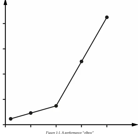
Reading performance graphs
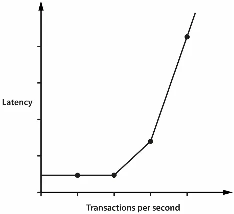
Figure 1-1. A performance “elbow”
The graph in Figure 1-1 shows sudden, unexpected degradation of
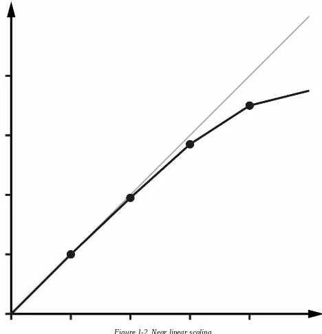
Figure 1-2. Near linear scaling
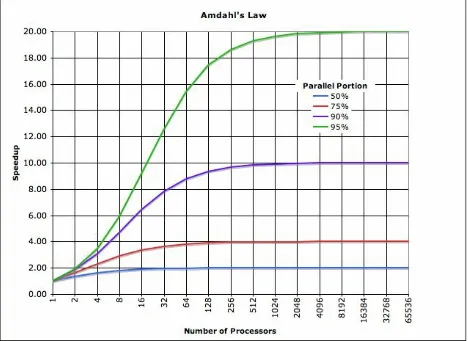
Figure 1-3. Amdahl’s Law
In Chapter 12 we will meet Amdahl’s Law, named for the famous computer scientist (and “father of the mainframe”) Gene Amdahl of IBM. Figure 1-3 shows a graphical representation of this fundamental constraint on scalability. It shows that whenever the workload has any piece at all that must be
performed in serial, linear scalability is impossible, and there are strict limits on how much scalability can be achieved. This justifies the commentary around Figure 1-2 - even in the best cases linear scalability is all but impossible to achieve.
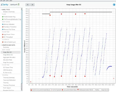
Figure 1-4. Healthy memory usage
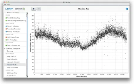
Figure 1-5. Stable allocation rate
Figure 1-6. Degrading latency under higher load
In the case where a system has a resource leak, it is far more common for it to manifest in a manner like that shown in Figure 1-6, where an observable (in this case latency) to slowly degrade as the load is ramped up.
In this chapter we have started to discuss what Java performance is and is not. We have introduced the fundamental topics of empirical science and
measurement, and introduced the basic vocabulary and observables that a good performance exercise will use. Finally, we have introduced some common cases that are often seen within the results obtained from
Overview
There is no doubt that Java is one of the largest technology platforms on the planet, boasting roughly 9-10 million Java developers. By design, many developers do not need to know about the low level intricacies of the platform they work with. This leads to a situation where developers only meet these aspects when a client complains about performance for the first time.
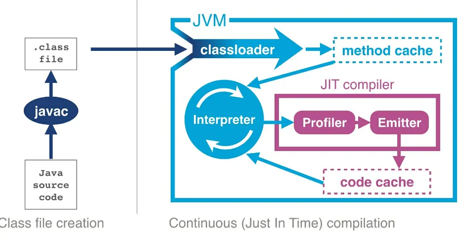
Code Compilation and Bytecode
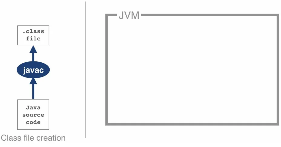
It is important to appreciate that Java code goes through a significant number of transformations before execution. The first is the compilation step using the Java Compiler javac, often invoked as part of a larger build process. The job of javac is to convert Java code into .class files that contain bytecode. It achieves this by doing a fairly straightforward translation of the Java source code, as shown in Figure 2-1. Very few optimizations are done during compilation by javac and the resulting bytecode is still quite
readable and recognisable as Java code when viewed in a disassembly tool, such as the standard javap.
Figure 2-1. Java class file compilation
Bytecode is an intermediate representation that is not tied to a specific machine architecture. Decoupling from the machine architecture provides portability, meaning developed software can run on any platform supported by the JVM and provides an abstraction from the Java language. This
NOTE
The Java language and the Java Virtual Machine are now to a degree independent, and so the J in JVM is potentially a little misleading, as the JVM can execute any JVM language that can produce a valid class file. In fact, Figure 2-1 could just as easily show the Scala compiler scalac generating bytecode for execution on the JVM.
Regardless of the source code compiler used, the resulting class file has a very well defined structure specified by the VM specification. Any class that is loaded by the JVM will be verified to conform to the expected format before being allowed to run.
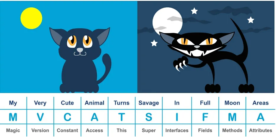
Table 2-1. Anatomy of a Class File
Component Description
Magic Number 0xCAFEBABE
Version of Class File Format The minor and major versions of the class file
Constant Pool Pool of constants for the class
Access Flags For example whether the class is abstract, static, etc.
This Class The name of the current class
Super Class The name of the super class
Interfaces Any interfaces in the class
Fields Any fields in the class
Methods Any methods in the class
Attributes Any attributes of the class (e.g. name of the sourcefile, etc.)
the version used to compile the class file. The major minor version is checked by the classloader to ensure compatibility, if these are not compatible an UnsupportedClassVersionError will be thrown at runtime indicating the runtime is a lower version than the compiled class file.
NOTE
Magic numbers provide a way for Unix environments to identify the type of a file
(whereas Windows will typically use the file extension). For this reason, they are difficult to change once decided upon. Unfortunately, this means that Java is stuck using the rather embarassing and sexist 0xCAFEBABE for the forseeable future.
The constant pool holds constant values in code for example names of classes, interfaces and field names. When the JVM executes code the
constant pool table is used to refer to values rather than having to rely on the layout of the class file at runtime.
Access flags are used to determine the modifiers applied to the class. The first part of the flag identifies whether a class is public followed by if it is final and cannot be subclassed. The flag also determines whether the class file represents an interface or an abstract class. The final part of the flag
represents whether the class file represents a synthetic class that is not present in source code, an annotation type or an enum.
The this class, super class and interface entries are indexes into the
constant pool to identify the type hierarchy belonging to the class. Fields and methods define a signature like structure including the modifiers that apply to the field or method. A set of attributes are then used to represent structured items for more complicated and non fixed size structures. For example, methods make use of the code attribute to represent the bytecode associated with that particular method.
Figure 2-2. mnemonic for class file structure
Taking a very simple code example it is possible to observe the effect of running javac:
Java ships with a class file disassembler called javap, allowing inspection of .class files. Taking the HelloWorld .class file and running javap -c HelloWorld gives the following output:
public class HelloWorld {
Code:
The overall layout describes the bytecode for HelloWorld class file, javap also has a -v option that provides the full classfile header information and constant pool details. The class file contains two methods, although only the single main method was supplied in the source file - this is the result of javac automatically adding a default constructor to the class.
The first instruction executed in the constructor is aload_0, which places the this reference onto the first position in the stack. The
invokespecial command is then called, which invokes an instance method that has specific handling for calling super constructors and the creation of objects. In the default constructor the invoke matches to the default constructor for Object as an override was not supplied.
NOTE
Opcodes in the JVM are concise and represent the type, the operation and the interaction between local variables, the constant pool and the stack.
(“if integer compare greater or equal”). The test only succeeds if the current integer is >= 10.
For the first few iterations, this comparison test fails and so we continue to instruction 8. Here the static method from System.out is resolved, followed by the loading of the Hello World String from the constant pool. The next invoke, invokevirtual is encountered, which invokes an
instance method based on the class. The integer is then incremented and goto is called to loop back to instruction 2. This process continues until the
Interpreting and Classloading
The JVM is a stack based interpreted machine. This means that rather than having registers (like a physical hardware CPU), it uses an execution stack of partial results, and performs calculations by operating on the top value (or values) of that stack.
The action of the JVM interpreter can be simply thought of a switch inside a while loop - processing each opcode independently of the last using the stack positions to hold intermediate values.
NOTE
As we will see when we delve into the internals of the Oracle / OpenJDK VM (HotSpot), the situation for real production-grade Java interpreters is a little more complex, but switch-inside-while is an acceptable mental model for the moment.
When our application is launched using the java HelloWorld command, the entry point into the application will be the main() method of
HelloWorld.class. In order to hand over control to this class, it must be loaded by the virtual machine before execution can begin.
To achieve this, the operating system starts the virtual machine process and almost immediately, the first in a chain of class loaders is initialised. This initial loader is known as the Bootstrap classloader, and contains classes in the core Java runtime. In current versions these are loaded from rt.jar, although this is changing in Java 9, as we will see in Chapter 13.
The Extension classloader is created next, it defines its parent to be the Bootstrap classloader, and will delegate to parent if needed. Extensions are not widely used, but can supply overrides and native code for specific
operating systems and platforms. Notably, the Nashorn Javascript runtime in Java 8 is loaded by the Extension loader.
loading in user classes from the defined classpath. Some texts unfortunately refer to this as the “System” classloader. This term should be avoided, for the simple reason tht it doesn’t load the system (the Bootstrap classloader does). The Application classloader is encountered extremely frequently, and it has the Extension loader as its parent.
Java loads in dependencies on new classes when they are first encountered during the execution of the program. If a class loader fails to find a class the behaviour is usually to delegate the lookup to the parent. If the chain of lookups reaches the bootstrap class loader and isn’t found a
ClassNotFoundException will be thrown. It is important that
developers use a build process that effectively compiles with the exact same classpath that will be used in Production, as this helps to mitigate this
potential issue.
Under normal circumstances Java only loads a class once and a Class object is created to represent the class in the runtime environment. However, it is important to realise that the same class can potentially be loaded twice by different classloaders. As a result class in the system is identified by the
Introducing HotSpot
Figure 2-3. The HotSpot JVM
In April 1999 Sun introduced one of the biggest changes to Java in terms of performance. The HotSpot virtual machine is a key feature of Java that has evolved to enable performance that is comparative to (or better than)
languages such as C and C++. To explain how this is possible, let’s delve a little deeper into the design of languages intended for application
development.
Language and platform design frequently involves making decisions and tradeoffs between desired capabilities. In this case, the division is between languages that stay “close to the metal” and rely on ideas such as “zero cost abstractions”, and languages that favour developer productivity and “getting things done” over strict low-level control.
C++ implementations obey the zero-overhead principle: What you don’t use, you don’t pay for. And further, what you do use, you couldn’t hand code any better.
The zero-overhead principle sounds great in theory, but it requires all users of the language to deal with the low-level reality of how operating systems and computers actually work. This is a significant extra cognitive burden that is placed upon developers that may not care about raw performance as a primary goal.
Not only that, but it also requires the source code to be compiled to platform-specific machine code at build time - usually called Ahead of Time (AOT) compilation. This is because alternative execution models such as
interpreters, virtual machines and portablity layers all are most definitely not zero overhead.
The principle also hides a can of worms in the phrase “what you do use, you couldn’t hand code any better”. This presupposes a number of things, not least that the developer is able to produce better code than an automated system. This is not a safe assumption at all. Very few people want to code in assembly language any more, so the use of automated systems (such as compilers) to produce code is clearly of some benefit to most programmers.
Java is a blue collar language. It’s not PhD thesis material but a language for a job.
James Gosling
Java has never subscribed to the zero-overhead abstraction philosophy. Instead, it focused on practicality and developer productivity, even at the expense of raw performance. It was therefore not until relatively recently, with the increasing maturity and sophistication of JVMs such as HotSpot that the Java environment became suitable for high-performance computing
applications.
HotSpot works by monitoring the application whilst it is running in interpreted mode and observing parts of code that are most frequently executed. During this analysis process programatic trace information is
captured that allows for more sophisticated optimisation. Once execution of a particular method passes a threshold the profiler will look to compile and optimize that section of code.
threshold is known as just-in-time compilation or JIT. One of the key benefits of JIT is having trace information that is collected during the interpreted phase, enabling HotSpot to make more informed optimisations. HotSpot has had hundreds of years (or more) of development attributed to it and new optimisations and benefits are added with almost every new release.
NOTE
After translation from Java source to bytecode and now another step of (JIT) compilation the code actually being executed has changed very significantly from the source code as written. This is a key insight and it will drive our approach to dealing with performance related investigations. JIT-compiled code executing on the JVM may well look nothing like the original Java source code.
The general picture is that languages like C++ (and the up-and-coming Rust) tend to have more predictable performance, but at the cost of forcing a lot of low-level complexity onto the user.
Note that “more predictable” does not necessarily mean “better”. AOT compilers produce code that may have to run across a broad class of
processors, and may not be able to assume that specific processor features are available.
Environments that use profile-guided optimization, such as Java, have the potential to use runtime information in ways that are simply impossible to most AOT platforms. This can offer improvements to performance, such as dynamic inlining and eliding virtual calls. HotSpot can also detect the precise CPU type it is running on at VM startup, and can use specific processor
features if available, for even higher performance. These are known as JVM “intrinsics” and are discussed in detail in Chapter 9.
The sophisticated approach that HotSpot takes is a great benefit to the
majority of ordinary developers, but this tradeoff (to abandon zero overhead abstractions) means that in the specific case of high performance Java
actually execute.
NOTE
Analysing the performance of small sections of Java code (“microbenchmarks”) is usually actually harder than analysing entire applications, and is a very specialist task that the majority of developers should not undertake. We will return to this subject in Chapter 5.
HotSpot’s compilation subsystem is one of the two most important
JVM Memory Management
In languages such as C, C\++ and Objective-C the programmer is responsible for managing the allocation and releasing of memory. The benefits of
managing your own memory and lifetime of objects are more deterministic performance and the ability to tie resource lifetime to the creation and
deletion of objects. This benefit comes at a cost - for correctness developers must be able to accurately account for memory.
Unfortunately, decades of practical experience showed that many developers have a poor understanding of idioms and patterns for management of
memory. Later versions of C\++ and Objective-C have improved this using smart pointer idioms in the core language. However at the time Java was created poor memory management was a major cause of application errors. This led to concern among developers and managers about the amount of time spent dealing with language features rather than delivering value for the business.
Java looked to help resolve the problem by introducing automatically
managed heap memory using a process known as Garbage Collection (GC). Simply put, Garbage Collection is a non-deterministic process that triggers to recover and resue no-longer needed memory when the JVM requires more memory for allocation.
However the story behind GC is not quite so simple or glib, and various algorithms for garbage collection have been developed and applied over the course of Java’s history. GC comes at a cost, when GC runs it often stops the world, which means whilst GC is in progress the application pauses. Usually these pause times are designed to be incredibly small, however as an
application is put under pressure these pause times can increase.
Threading and the Java Memory Model
One of the major advances that Java brought in with its first version is direct support for multithreaded programming. The Java platform allows the
developer to create new threads of execution. For example, in Java 8 syntax:
Thread t = new Thread(() -> {System.out.println("Hello World!");}); t.start();
This means that all Java programs are inherently multithreaded (as is the JVM). This produces additional, irreducible complexity in the behaviour of Java programs, and makes the work of the performance analyst even harder. Java’s approach to multithreading dates from the late 1990s and has these fundamental design principles:
All threads in a Java process share a single, common garbage-collected heap
Any object created by one thread can be accessed by any other thread that has a reference to the object
Objects are mutable by default - the values held in object fields can be changed unless the programmer explicitly uses the final keyword to mark them as immutable.
The Java Memory Model (JMM) is a formal model of memory that explains how different threads of execution see the changing values held in objects. That is, if threads A and B both have references to object obj, and thread A alters it, what happens to the value observed in thread B.
The JVM and the operating system
Java and the JVM provide a portable execution environent that is independent of the operating system. This is implemented by providing a common
interface to Java code. However, for some fundamental services, such as thread scheduling (or even something as mundane as getting the time from the system clock), the underlying operating system must be accessed. This capability is provided by native methods, which are denoted by the keyword native. They are written in C, but are accessible as ordinary Java methods. This interface is referred to as the Java Native Interface (JNI). For example, java.lang.Object declares these non-private native methods:
public final native Class<?> getClass(); public native int hashCode();
protected native Object clone() throws CloneNotSupportedException; public final native void notify();
public final native void notifyAll();
public final native void wait(long timeout) throws InterruptedException;
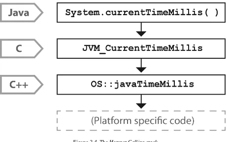
As all these methods deal with relatively low-level platform concerns, let’s look at a more straightforward and familiar example - getting the system time.
Consider the os::javaTimeMillis() function. This is the (system-specific) code responsible for implementing the Java
Figure 2-4. The Hotspot Calling stack
As you can see in Figure 2-4, the native
System.currentTimeMillis() method is mapped to the JVM entry point method JVM_CurrentTimeMillis. This mapping is achieved via the JNI Java_java_lang_System_registerNatives mechanism contained in java/lang/System.c.
JVM_CurrentTimeMillis is essentially a call to the C+\+ method
os::javaTimeMillis() wrapped in a couple of OpenJDK macros. This method is defined in the os namespace, and is unsurprisingly operating
system-dependent. Definitions for this method are provided by the OS-specific subdirectories of source code within OpenJDK.
This demonstrates how the platform-independent parts of Java can call into services that are provided by the underlying operating system and hardware. In Chapter 3 we will discuss some details of how operating systems and hardware work. This is to provide necessary background for the Java
Chapter 3. Hardware &
Operating Systems
Why should Java developers care about Hardware?
For many years the computer industry has been driven by Moore’s Law, a hypothesis made by Intel founder, Gordon Moore, about long-term trends in processor capability. The law (really an observation or extrapolation) can be framed in a variety of ways, but one of the most usual is:
The number of transistors on a mass-produced chip roughly doubles every 18 months
Gordon Moore
This phenomenon represents an exponential increase in computer power over time. It was originally cited in 1965, so represents an incredible long-term trend, almost unparalleled in the history of human development. The effects of Moore’s Law have been transformative in many (if not most) areas of the modern world.
NOTE
The death of Moore’s Law has been repeatedly proclaimed for decades now. However, there are very good reasons to suppose that, for all practical purposes, this incredible progress in chip technology has (finally) come to an end.
The net result of this huge increase in the performance available to the
ordinary application developer has been the blossoming of complex software. Software applications now pervade every aspect of global society. Or, to put it another way:
Software is eating the world. Marc Andreessen
As we will see, Java has been a beneficiary of the increasing amount of computer power. The design of the language and runtime has been well-suited (or lucky) to make use of this trend in processor capability. However, the truly performance-conscious Java programmer needs to understand the principles and technology that underpins the platform in order to make best use of the available resources.
Introduction to Modern Hardware
Many universty courses on hardware architectures still teach a simple-to-understand, “classical” view of hardware. This “motherhood and apple pie” view of hardware focuses on a simple view of a register-based machine, with arithmetic and logic operations, load and store operations.
Since then, however, the world of the application developer has, to a large extent, revolved around the Intel x86 / x64 architecture. This is an area of technology that has undergone radical change and many advanced features now form important parts of the landscape. The simple mental model of a processor’s operation is now completely incorrect, and intuitive reasoning based on it is extremely liable to lead to utterly wrong conclusions.
Memory
As Moore’s Law advanced, the exponentially increasing number of
transistors was initially used for faster and faster clock speed. The reasons for this are obvious - faster clock speed means more instructions completed per second. Accordingly, the speed of processors has advanced hugely, and the 2+ GHz processors that we have today are hundreds of times faster than the original 4.77 MHz chips found in the first IBM PC.
However, the increasing clock speeds uncovered another problem. Faster chips require a faster stream of data to act upon. As Figure 3-1 1 shows, over
time main memory could not keep up with the demands of the processor core for fresh data.
Figure 3-1. Speed of memory and transistor counts
on the CPU that are slower than CPU registers, but faster than main memory. The idea is for the CPU to fill the cache with copies of often-accessed
memory locations rather than constantly having to re-address main memory. Modern CPUs have several layers of cache, with the most-often-accessed caches being located close to the processing core. The cache closest to the CPU is usually called L1, with the next being referred to as L2, and so on. Different processor architectures have a varying number, and configuration, of caches, but a common choice is for each execution core to have a
dedicated, private L1 and L2 cache, and an L3 chache that is shared across some or all of the cores. The effect of these caches in speeding up access times is shown in Figure 3-2 2.
Figure 3-2. Access times for various types of memory
Memory Caches
Modern hardware does introduce some new problems in terms of determining how memory is fetched into and written back from cache. This is known as a “cache consistency protocol”.
At the lowest level, a protocol called MESI (and its variants) is commonly found on a wide range of processors. It defines four states for any line in a cache. Each line (usually 64 bytes) is either:
Modified (but not yet flushed to main memory)
Exclusive (only present here, but does match main memory)
Shared (may also be present in other caches, matches main memory)
Invalid (may not be used, will be dropped as soon as practical)
Table 3-1.
The idea of the protocol is that multiple processors can simultenously be in the Shared state. However, if a processor transitions to any of the other valid states (Exclusive or Modified), then this will force all the other processors into the Invalid state. This is shown in Table 3-1
Figure 3-3. MESI state transition diagram
Originally, processors wrote every cache operation directly into main memory. This was called “write-through” behavior, but it was and is very inefficient, and required a large amount of bandwidth to memory. More recent processors also implement “write-back” behavior, where traffic back to main memory is significantly reduced.
terms of the bandwidth to memory. The “burst rate”, or theoretical maximum is based on several factors:
Clock frequency of memory
The width of the memory bus (usually 64 bits)
Number of interfaces (usually 2 in modern machines)
This is multiplied by 2 in the case of DDR RAM (DDR stands for “double data rate”). Applying the formula to 2015 commodity hardware gives a theoretical maximum write speed of 8-12GB/s. In practice, of course, this could be limited by many other factors in the system. As it stands, this gives a modestly useful value to allow us to see how close the hardware and software can get.
Let’s write some simple code to exercise the cache hardware:
private void touchEveryLine() {
Intuitively, touchEveryItem() “does 16 times as much work” as touchEveryLine(), as 16 times as many data items must be updated. However, the point of this simple example is to show how badly intuition can lead us astray when dealing with JVM performance. Let’s look at some
sample output from the Caching class, as shown in Figure 3-4:
Figure 3-4. Time elapsed for Caching example
The graph shows 100 runs of each function, and is intended to show several different effects. Firstly, notice that the results for both functions are
Instead, the dominant effect of this code is to exercise the memory bus, by transferring the contents of the array from main memory, into the cache to be operated on by touchEveryItem() and touchEveryLine().
In terms of the statistics of the numbers, although the results are reasonably consistent, there are individual outliers that are 30-35% different from the median value.
Overall, we can see that each iteration of the simple memory function takes around 3 milliseconds (2.86ms on average) to traverse a 100M chunk of memory, giving an effective memory bandwidth of just under 3.5GB per second. This is less than the theoretical maximum, but is still a reasonable number.
NOTE
Modern CPUs have a hardware prefetcher, that can detect predictable patterns in data access (usually just a regular “stride” through the data). In this example, we’re taking advantage of that fact in order to get closer to a realistic maximum for memory access bandwidth.
Modern Processor Features
Translation Lookaside Buffer
One very important use is in a different sort of cache - the Translation Lookaside Buffer (TLB). This acts as a cache for the page tables that map virtual memory addresses to physical addresses. This greatly speeds up a very frequent operation - access to the physical address underlying a virtual
address.
NOTE
There’s a memory-related software feature of the JVM that also has the acronym TLB (as we’ll see later). Always check which features is being discussed when you see TLB mentioned.
Branch Prediction and Speculative Execution
One of the advanced processor tricks that appears on modern processors is branch prediction. This is used to prevent the processor having to wait to evaluate a value needed for a conditional branch. Modern processors have multistage instruction pipelines. This means that the execution of a single CPU cycle is broken down into a number of separate stages. There can be several instructions in-flight (at different stages of execution) at once.
In this model, a conditional branch is problematic, because until the condition is evaluated, it isn’t known what the next instruction after the branch will be. This can cause the processor to stall for up to 20 cycles, as it effectively empties the multi-stage pipeline behind the branch.
To avoid this, the processor can dedicate transistors to building up a heuristic to decide which branch is more likely to be taken. Using this guess, the CPU fills the pipeline based on a gamble - if it works, then the CPU carries on as though nothing had happened. If it’s wrong, then the partially executed
Hardware Memory Models
The core question about memory that must be answered in a multicore system is “How can multiple different CPUs access the same memory location safely?”.
The answer to this question is highly hardware dependent, but in general, javac, the JIT compiler and the CPU are all allowed to make changes to the order in which code executes, provided that it doesn’t affect the outcome as observed by the current thread.
For example, let’s suppose we have a piece of code like this:
myInt = otherInt; intChanged = true;
There is no code between the two assignments, so the executing thread
doesn’t need to care about what order they happen in, and so the environment is at liberty to change the order of instructions.
However, this could mean that in another thread that has visibility of these data items, the order could change, and the value of myInt read by the other thread could be the old value, despite intChanged being seen to be true. This type of reordering (store moved after store) is not possible on x86 chips, but as Table 3-2 shows, there are other architectures where it can, and does, happen.
Table 3-2. Hardware memory support
ARMv7 POWER SPARC x86 AMD64 zSeries
Loads moved after loads Y Y - - -
-Loads moved after stores Y Y - - -
-Stores moved after stores Y Y - - -
-Stores moved after loads Y Y Y Y Y Y
-Atomic moved with stores Y Y - - -
-Incoherent instructions Y Y Y Y - Y
In the Java environment, the Java memory model (JMM) is explicitly designed to be a weak model to take into account the differences in
consistency of memory access between processor types. Correct use of locks and volatile access is a major part of ensuring that multithreaded code works properly. This is a very important topic that we will return to later in the book, in Chapter 12.
There has been a trend in recent years for software developers to seek greater understanding of the workings of hardware in order to derive better
Operating systems
The point of an operating system is to control access to resources that must be shared between multiple executing processes. All resources are finite, and all processes are greedy, so the need for a central system to arbitrate and meter access is essential. Among these scarce resources, the two most important are usually memory and CPU time.
Virtual addressing via the memory management unit and its page tables are the key feature that enables access control of memory, and prevents one process from damaging the memory areas owned by another.
The Scheduler
Figure 3-5. Thread Lifecycle
In this relatively simple view, the OS scheduler moves threads on and off the single core in the system. At the end of the time quantum (often 10ms or 100ms in older operating systems), the scheduler moves the thread to the back of the run queue to wait until it reaches the front of the queue and is eligible to run again.
If a thread wants to voluntarily give up its time quantum it can do so either for a fixed amount of time (via sleep()), or until a condition is met (using wait()). Finally, a thread can also block on I/O or a software lock.
When meeting this model for the first time, it may help to think about a machine that has only a single execution core. Real hardware is, of course, more complex and virtually any modern machine will have multiple cores, and this allows for true simultaneous execution of multiple execution paths. This means that reasoning about execution in a true multiprocessing
environment is very complex and counter-intuitive.
comes to the front of the run queue again. This combines with the fact that CPU is a scarce resource to give us the fact that “code is waiting more often than it is running”.
This means that the statistics we want to generate from processes that we actually want to observe are affected by the behavior of other processes on the systems. This “jitter” and the overhead of scheduling is a primary cause of noise in observed results. We will discuss the statistical properties and handling of real results in Chapter 5.
One of the easiest ways to see the action and behavior of a scheduler is to try to observe the overhead imposed by the OS to achieve scheduling. The
following code executes 1000 separate 1 ms sleeps. Each of these sleeps will involve the thread being sent to the back of the run queue, and having to wait for a new time quantum. So, the total elapsed time of the code gives us some idea of the overhead of scheduling for a typical process.
long start = System.currentTimeMillis();
Running this code will cause wildly divergent results, depending on operating system. Most Unixes will report 10-20% overhead. Earlier versions of
Windows had notoriously bad schedulers - with some versions of Windows XP reporting up to 180% overhead for scheduling (so that a 1000 sleeps of 1 ms would take 2.8s). There are even reports that some proprietary OS
vendors have inserted code into their releases in order to detect benchmarking runs and cheat the metrics.
A Question of Time
Despite the existence of industry standards such as POSIX, different
operating systems can have very different behaviors. For example, consider the os::javaTimeMillis() function. In OpenJDK this contains the OS-specific calls that actually do the work and ultimately supply the value to be eventually returned by Java’s System.currentTimeMillis() method.
As we discussed in Section 2.6, as this relies on functionality that has to be provided by the host operating system, this has to be implemented as a native method. Here is the function as implemented on BSD Unix (e.g. for Apple’s OS X operating system):
jlong os::javaTimeMillis() { timeval time;
int status = gettimeofday(&time, NULL); assert(status != -1, "bsd error");
return jlong(time.tv_sec) * 1000 + jlong(time.tv_usec / 1000); }
The versions for Solaris, Linux and even AIX are all incredibly similar to the BSD case, but the code for Microsoft Windows is completely different:
jlong os::javaTimeMillis() { if (UseFakeTimers) {
return fake_time++; } else {
FILETIME wt;
GetSystemTimeAsFileTime(&wt); return windows_to_java_time(wt); }
}
Windows uses a 64-bit FILETIME type to store the time in units of 100ns elapsed since the start of 1601, rather than the Unix timeval structure. Windows also has a notion of the “real accuracy” of the system clock,
machines.
Context Switches
Context switches can be a very costly operation, whether between user threads or from user mode into kernel mode. The latter case is particularly important, because a user thread may need to swap into kernel mode in order to perform some function partway through its time slice. However, this
switch will force instruction and other caches to be emptied, as the memory areas accessed by the user space code will not normally have anything in common with the kernel.
A context switch into kernel mode will invalidate the TLBs and potentially other caches. When the call returns, these cashes will have to be refilled and so the effect of a kernel mode switch persists even after control has returned to user space. This causes the true cost of a system call to be masked, as can be seen in Figure 3-6 3.
Figure 3-6. Impact of a system call
that is used to speed up syscalls that do not really require kernel privileges. It achieves this speed increase by not actually performing a context switch into kernel mode. Let’s look at an example to see how this works with a real syscall.
A very common Unix system call is gettimeofday(). This returns the “wallclock time” as understood by the operating system. Behind the scenes, it is actually just reading a kernel data structure to obtain the system clock time. As this is side-effect free, it does not actually need privileged access.
If we can use vDSO to arrange for this data structure to be mapped into the address space of the user process, then there’s no need to perform the switch to kernel mode, and the refill penalty shown in Figure 3-6 does not have to be paid.
A simple system model
In this section we describe a simple model for describing basic sources of possible performance problems. The model is expressed in terms of operating system observables of fundamnetal subsystems and can be directly related back to the outputs of standard Unix command line tools.
Figure 3-7. Simple system model
The model is based around a simple conception of a Java application running on a Unix or Unix-like operating system. Figure 3-7 shows the basic
components of the model, which consist of:
The hardware and operating system the application runs on
The JVM (or container) the application runs in
The application code itself
The incoming request traffic that is hitting the application
Basic Detection Strategies
One definition for a well-performing application is that efficient use is being made of system resources. This includes CPU usage, memory and network or I/O bandwidth. If an application is causing one or more resource limits to be hit, then the result will be a performance problem.
It is also worth noting that the operating system itself should not normally be a major contributing factor to system utilisation. The role of an operating system is to manage resources on behalf of user processes, not to consume them itself. The only real exception to this rule is when resources are so scarce that the OS is having difficulty allocating anywhere near enough to satisfy user requirements. For most modern server-class hardware, the only time this should occur is when I/O (or occassionally memory) requirements greatly exceed capability.
A key metric for application performance is CPU utilisation. CPU cycles are quite often the most critical resource needed by an application, and so
efficient use of them is essential for good performance. Applications should be aiming for as close to 100% usage as possible during periods of high load.
NOTE
When analysing application performance, the system must be under enough load to exercise it. The behavior of an idle application is usually meaningless for performance work.
ben@janus:~$ vmstat 1
The parameter 1 following vmstat indicates that we want vmstat to provide ongoing output (until interrupted via Ctrl-C) rather than a single snapshot. New output lines are printed, every second, which enables a performance engineer to leave this output running (or capturing it into a log) whilst an initial performance test is performed.
The output of vmstat is relatively easy to understand, and contains a large amount of useful information, divided into sections.
1. The first two columns show the number of runnable and blocked processes.
2. In the memory section, the amount of swapped and free memory is shown, followed by the memory used as buffer and as cache.
3. The swap section shows the memory swapped from and to disk. Modern server class machines should not normally experience very much swap activity.
4. The block in and block out counts (bi and bo) show the number of 512-byte blocks that have been received from, and sent to a block (I/O) device.
6. The CPU section contains a number of directly relevant metrics, expressed as percentages of CPU time. In order, they are user time (us), kernel time (sy, for “system time”), idle time (id), waiting time (wa) and the “stolen time” (st, for virtual machines).
Over the course of the remainder of this book, we will meet many other, more sophisticated tools. However, it is important not to neglect the basic tools at our disposal. Complex tools often have behaviors that can mislead us, whereas the simple tools that operate close to processes and the operating system can convey simple and uncluttered views of how our systems are actually behaving.
Context switching
In Section 3.4.3, we discussed the impact of a context switch, and saw the potential impact of a full context switch to kernel space in Figure 3-6. However, whether between user threads or into kernel space, context switches introduce unavoidable wastage of CPU resources.
A well-tuned program should be making maximum possible use of its
resources, especially CPU. For workloads which are primarily dependent on computation (“CPU-bound” problems), the aim is to achieve close to 100% utilisation of CPU for userland work.
To put it another way, if we observe that the CPU utilisation is not
approaching 100% user time, then the next obvious question is to ask why not? What is causing the program to fail to achieve that? Are involuntary context switches caused by locks the problem? Is it due to blocking caused by I/O contention?
The vmstat tool can, on most operating systems (especially Linux), show the number of context switches occurring, so on a vmstat 1 run, the
analyst will be able to see the real-time effect of context switching. A process that is failing to achieve 100% userland CPU usage and is also displaying high context-switch rate is likely to be either blocked on I/O or thread lock contention.
Garbage Collection
As we will see in Chapter 7, in the HotSpot JVM (by far the most commonly used JVM), memory is allocated at startup and managed from within user space. That means, that system calls such as sbrk() are not needed to allocate memory. In turn, this means that kernel switching activity for garbage collection is quite minimal.
Thus, if a system is exhibiting high levels of system CPU usage, then it is definitely not spending a significant amount of its time in GC, as GC activity burns user space CPU cycles and does not impact kernel space utilization. On the other hand, if a JVM process is using 100% (or close to) of CPU in user space, then garbage collection is often the culprit. When analysing a performance problem, if simple tools (such as vmstat) show consistent 100% CPU usage, but with almost all cycles being consumed by userspace, then a key question that should be asked next is: “Is it the JVM or user code that is responsible for this utilization?”. In almost all cases, high userspace
utilization by the JVM is caused by the GC subsystem, so a useful rule of thumb is to check the GC log & see how often new entries are being added to it.
Garbage collection logging in the JVM is incredibly cheap, to the point that even the most accurate measurements of the overall cost cannot reliably distinguish it from random background noise. GC logging is also incredibly useful as a source of data for analytics. It is therefore imperative that GC logs be enabled for all JVM processes, especially in production.
I/O
File I/O has traditionally been one of the murkier aspects of overall system performance. Partly this comes from its closer relationship with messy physical hardware, with engineers making quips about “spinning rust” and similar, but it is also because I/O lacks as clean abstractions as we see elsewhere in operating systems.
In the case of memory, the elegance of virtual memory as a separation mechanism works well. However, I/O has no comparable abstraction that provides suitable isolation for the application developer.
Fortunately, whilst most Java programs involve some simple I/O, the class of applications that make heavy use of the I/O subsystems is relatively small, and in particular, most applications do not simultenously try to saturate I/O at the same time as either CPU or memory.
Not only that, but established operational practice has led to a culture in which production engineers are already aware of the limitations of I/O, and actively monitor processes for heavy I/O usage.
For the performance analyst / engineer, it suffices to have an awareness of the I/O behavior of our applications. Tools such as iostat (and even vmstat) have the basic counters (e.g. blocks in or out) that are often all we need for basic diagnosis, especially uf we make the assumption that only one I/O-intensive application is present per host.
Finally, it’s worth mentioning one aspect of I/O that is becoming more
Kernel Bypass I/O
Figure 3-8. Kernel Bypass I/O
NOTE
In some ways, this is reminiscent of Java’s New I/O (NIO) API that was introduced to allow Java I/O to bypass the Java heap and work directly with native memory and underlying I/O.
increasingly commonly implemented in systems that require very high-performance I/O.
In this chapter so far we have discussed operating systems running on top of “bare metal”. However, increasingly, systems run in virtualised
Virtualisation
Figure 3-9. Virtualisation of operating systems
A full discussion of virtualisation, the relevant theory and its implications for application performance tuning would take us too far afield. However, some mention of the differences that virtualisation causes seems approriate,
especially given the increasing amount of applications running in virtual, or cloud environments.
Although virtualisation was originally developed in IBM mainframe environments as early as the 1970s, it was not until recently that x86
architectures were capable of supporting “true” virtualisation. This is usually characterized by these three conditions:
Programs running on a virtualized OS should behave essentially the same as when running on “bare metal” (i.e. unvirtualized)
The overhead of the virtualization must be as small as possible, and not a significant fraction of execution time.
In a normal, unvirtualized system, the OS kernel runs in a special, privileged mode (hence the need to switch into kernel mode). This gives the OS direct access to hardware. However, in a virtualized system, direct access to
hardware by a guest OS is disallowed.
One common approach is to rewrite the privileged instructions in terms of unprivileged instructions. In addition, some of the OS kernel’s data structures need to be “shadowed” to prevent excessive cache flushing (e.g. of TLBs) during context switches.
Some modern Intel-compatible CPUs have hardware features designed to improve the performance of virtualized OSs. However, it is apparent that even with hardware assists, running inside a virtual environment presents an additional level of complexity for performance analysis and tuning.
In the next chapter we will introduce the core methodology of performance tests. We will discuss the primary types of performance tests, the tasks that need to be undertaken and the overall lifecycle of performance work. We will also catalogue some common best practices (and antipatterns) in the
performance space.
From Computer Architecture: A Quantitative Approach by Hennessy, et al.
Access times shown in terms of number of clock cycles per operation, provided by Google Image reproduced from “FlexSC: Flexible System Call Scheduling with Exception-Less System Calls” by Soares & Stumm
1
Chapter 4. Performance Testing
Patterns and Antipatterns
Performance testing is undertaken for a variety of different reasons. In this chapter we will introduce the different types of test that a team may wish to execute, and discuss best practices for each type.
In the second half of the chapter, we will outline some of the more common antipatterns that can plague a performance test or team, and explain
Types of Performance Test
Performance tests are frequently conducted for the wrong reasons, or
conducted badly. The reasons for this vary widely, but are frequently caused by a failure to understand the nature of performance analysis, and a belief that “something is better than nothing”. As we will see repeatedly, this belief is often a dangerous half-truth at best.
One of the more common mistakes is to speak generally of “performance testing” without engaging with the specifics. In fact, there are a fairly large number of different types of large-scale performance tests that can be performed on a system.
NOTE
Good performance tests are quantitative. They ask questions that have a numeric answer that can be handled as an experimental output, and subjected to statistical analysis.
The types of performance tests we will discuss in this book usually have mostly independent (but somewhat overlapping) goals, so care should be taken when thinking about the domain of any given single test. A good rule-of-thumb when planning a performance test is simply to write down (&
confirm to management / the customer) the quantitative questions that the test is intended to answer, and why they are important for the application under test.
Some of the most common test types, and an example question for each are given below.
Latency Test - what is the end-to-end transaction time?
Throughput Test - how many concurrent transactions can the current system capacity deal with?
Stress Test - what is the breaking point of the system?
Endurance Test - what performance anomalies are discovered when the system is run for an extended period?
Capacity Planning Test - Does the system scale as expected when additional resources are added?
Degradation - What happens when the system is partially failed?
Latency Test
This is one of the most common types of performance test, usually because it can be closely related to a system observable that is of direct interest to
management - how long are our customers waiting for a transaction (or a page load). This is a double-edged sword, as because the quantitative question that a latency test seeks to answer seems so obvious, that it can obscure the necessity of identifying quantitative questions for other types of performance tests.
NOTE
The goal of a latency tuning exercise is usually to directly improve user experience.
Throughput Test
Throughput is probably the second most common quantity to be the subject of a performance exercise. It can even be thought of as dual to latency, in some senses.
For example, when conducting a latency test, it is important to state (and control) the concurrent transactions ongoing when producing a distribution of latency results.
NOTE
The observed latency of a system should be stated at known and controlled throughput levels.
Load Test
Stress Test
One way to think about a stress test is as a way to determine how much spare headroom the system has. The test typically proceeds by placing the system into a steady state of transactions - that is a specified throughput level (often current peak). The test then ramps up the concurrent transactions slowly, until the system observables start to degrade.
Endurance Test
Some problems only manifest over much longer periods (often measured in days). These include slow memory leaks, cache pollution and memory fragmentation (especially for applications that use the CMS garbage collector, which may eventually suffer “Concurrent Mode Failure” - see Section 8.3).
To detect these types of issue, an Endurance Test (also known as a Soak Test) is the usual approach. These are run at average (or high) utilisation, but
within observed loads for the system. During the test resource levels are closely monitored and breakdowns or exhaustions of resources are looked for.