ISBN: 0-13-977430-0
Copyright 1999 by Prentice-Hall PTR
Copyright 2000 by Chrysalis Software Corporation
Would you like to discuss interesting topics with intelligent people? If
so, you might be interested in
Colloquy
, the world's first internet-based
high-IQ society. I'm one of the Regents of this society, and am responsible
for the email list and for membership applications. Application instructions
are available
here
.
Imagine that you are about to finish a relatively large program, one that has taken a few weeks or months to write and debug. Just as you are putting the finishing touches on it, you discover that it is either too slow or runs out of memory when you feed it a realistic set of input data. You sigh, and start the task of optimizing it.
But why optimize? If your program doesn't fit in memory, you can just get more memory; if it is too slow, you can get a faster processor.
I have written Optimizing C++ because I believe that this common attitude is incorrect, and that a knowledge of optimization is essential to a professional programmer. One very
important reason is that we often have little control over the hardware on which our programs are to be run. In this situation, the simplistic approach of adding more hardware is not feasible.
Optimizing C++ provides working programmers and those who intend to be working programmers with a practical, real-world approach to program optimization. Many of the optimization techniques presented are derived from my reading of academic journals that are, sadly, little known in the programming community. This book also draws on my nearly 30 years of experience as a programmer in diverse fields of application, during which I have become increasingly concerned about the amount of effort spent in reinventing optimization techniques rather than applying those already developed.
The first question you have to answer is whether your program needs optimization at all. If it does, you have to determine what part of the program is the culprit, and what resource is being overused. Chapter 1 indicates a method of attack on these problems, as well as a real-life example.
All of the examples in this book were compiled with both Microsoft's Visual C++ 5.0 and the DJGPP compiler, written and copyrighted by DJ Delorie. The latter compiler is available here. The source code for the examples is available here. If you want to use DJGPP, I recommend that you also get RHIDE, an integrated development environment for the DJGPP compiler, written and copyrighted by Robert Hoehne, which is available here.
All of the timings and profiling statistics, unless otherwise noted, were the result of running the corresponding program compiled with Visual C++ 5.0 on my Pentium II 233 Megahertz machine with 64 megabytes of memory.
I am always happy to receive correspondence from readers. If you wish to contact me, the best way is to visit my WWW home page.
If you prefer, you can email me.
In the event that you enjoy this book and would like to tell others about it, you might want to write an on-line review on Amazon.com, which you can do here.
I should also tell you how the various typefaces are used in the book. HelveticaNarrow is used for program listings, for terms used in programs, and for words defined by the C++ language. Italics are used primarily for technical terms that are found in the glossary, although they are also used for emphasis in some places. The first time that I use a particular technical term that you might not know, it is in bold face.
Dedication
Acknowledgements Prologue
A Supermarket Price Lookup System A Mailing List System
Cn U Rd Ths (Qkly)? A Data Compression Utility
Free at Last: An Efficient Method of Handling Variable-Length Records Heavenly Hash: A Dynamic Hashing Algorithm
Zensort: A Sorting Algorithm for Limited Memory Mozart, No. Would You Believe Gershwin? About the Author
Acknowledgements
I'd like to thank all those readers who have provided feedback on the first two editions of this book, especially those who have posted reviews on Amazon.com; their contributions have made this a better book.
I'd also like to thank Jeff Pepper, my editor at Prentice-Hall, for his support and encouragement. Without him, this third edition would never have been published.
Finally, I would like to express my appreciation to John P. Linderman at AT&T Labs Research for his help with the code in the chapter on sorting immense files.
Prologue
Introduction to Optimization
What is optimization anyway? Clearly, we have to know this before we can discuss how and why we should optimize programs.
Definition
Optimization is the art and science of modifying a working computer program so that it makes more efficient use of one or more scarce resources, primarily memory, disk space, or time. This definition has a sometimes overlooked but very important corollary (The First Law of Optimization): The speed of a nonworking program is irrelevant.
Algorithms Discussed
Radix40 Data Representation, Lookup Tables1
Deciding Whether to Optimize
Suppose you have written a program to calculate mortgage payments; the yearly run takes ten minutes. Should you spend two hours to double its speed? Probably not, since it will take twenty-four years to pay back the original investment of time at five minutes per year.2 On the other hand, if you run a program for three hours every working day, even spending thirty hours to double its speed will pay for itself in only twenty working days, or about a month. Obviously the latter is a much better candidate for optimization. Usually, of course, the situation is not nearly so unambiguous: even if your system is overloaded, it may not be immediately apparent which program is responsible.3 My general rule is not to optimize a program that performs satisfactorily. If you (or the intended users) don't become impatient while waiting for it to finish, don't bother. Of course, if you just feel like indulging in some recreational optimization, that's another matter.
Assuming that our programs are too big, or too slow, why don't we just add more memory or a faster processor? If that isn't possible today, then the next generation of processors should be powerful enough to spare us such concerns.
Let's examine this rather widely held theory. Although the past is not an infallible guide to the future, it is certainly one source of information about what happens when technology changes. A good place to start is to compare the computers of the late 1970's with those of the late 1990's.
The first diskette-based computer I ever owned was a Radio Shack TRS-80 Model IIITM, purchased in 1979.4 It had a 4 MHz Z80TM processor, 48 Kbytes of memory, and BasicTM in ROM. The diskettes held about 140 Kbytes apiece. Among the programs that were available for this machine were word processors, assemblers, debuggers, data bases, and games. While none of these were as advanced as the ones that are available today on 80x86 or 680x0 machines, most of the basic functions were there.
The Pentium IITM machines of today have at least 1000 times as much memory and 20000 times as much disk storage and are probably 1000 times as fast. Therefore, according to this theory, we should no longer need to worry about efficiency.
Recently, however, several of the major microcomputer software companies have had serious performance problems with new software releases of both application programs and system programs, as they attempted to add more and more features to those available in the previous versions.5 This illustrates what I call the Iron Law of Programming: whenever more resources are made available, a more ambitious project is attempted. This means that optimal use of these resources is important no matter how fast or capacious the machine.
Why Optimization Is Often Neglected
In view of this situation, why has optimization of application programs not gained more attention? I suspect that a major reason is the tremendous and continuing change in the relative costs of programming time and computer hardware. To illustrate this, let us examine two situations where the same efficiency improvement is gained, but the second example occurs after twenty years of technological improvement.
In the early 1970's a programmer's starting salary was about $3 per hour, and an hour of timesharing connect time cost about $15. Therefore, if a program originally took one hour to run every day, and the programmer spent a week to reduce this time by 20%, in about eight weeks the increased speed would have paid for the programmer's time.
In the late 1990's, the starting salary is in the vicinity of $15 per hour, and if we assume that the desktop computer costs $2500 and is amortized over three years, the weekly cost of running the unoptimized program is about $2.00. Holding the other assumptions constant, the optimization payback time is about 30 years!6 This long-term trend seems to favor hardware
optimization payback time is about 30 years!6 This long-term trend seems to favor hardware solutions for performance problems over the investment of programming effort. However, the appropriate strategy for performance improvement of a program depends on how much control you have over the hardware on which the program will run. The less control you have over the hardware, the greater the advantage of software solutions to performance problems, as
illustrated by the situations below.
Considering a Hardware Solution
While every optimization problem is different, here are some general guidelines that can help you decide whether adding hardware to help you with your performance problems makes sense.
1. If you are creating a system that includes both software and hardware, and you can improve the functioning of the program, ease maintenance, or speed up development at a small additional expense for extra hardware resources, you should almost certainly do so.
A few years ago, I was involved in a classic example of this situation. The project was to create a point-of-sale system, including specialized hardware and programs, that tied a number of terminals into a common database. Since the part of the database that had to be accessed rapidly could be limited to about 1 1/2 megabytes, I suggested that we put enough memory in the database server machine to hold the entire database. That way, the response time would be faster than even a very good indexing system could provide, and the programming effort would be greatly reduced. The additional expense came to about $150 per system, which was less than 3% of the price of the system. Of course, just adding hardware doesn't always mean that no software optimization is needed. In this case, as you will see below, adding the hardware was only the beginning of the optimization effort.
2. If you are writing programs for your own use on one computer, and you can afford to buy a machine powerful enough to perform adequately, then you might very well
purchase such a machine rather than optimizing the program.7
3. If you are writing a program that will be running on more than one computer, even if it is only for internal use at your company, the expense and annoyance of requiring the other users to upgrade their computers may outweigh the difficulty of optimization.
5. If your program is to be sold in the open market to run on standard hardware, you must try to optimize it. Otherwise, the users are likely to reject the program.
An excellent example of what happens when you try to make a number of users upgrade their computers is the relatively disappointing sales record (as of this writing) of the Windows NTTM operating system.
In order to get any reasonable performance under version 4.0 of Windows NT (the latest extant as of this writing), you need at least 64 megabytes of memory and a Pentium II/233 processor. Since almost the only people who have such machines are professional software developers, the sales of this program to other users have been much smaller than expected.
Categories of Optimization
There are two broad categories of optimization: using a better algorithm, and improving the implementation of the algorithm we are already using. Generally, we should replace an algorithm by a better one as soon as possible, as this usually does not hinder understanding or later modification of the program. An example is the use of a distribution counting sort (see Chapter mail.htm) in preference to Quicksort. Of course, if we employ these efficient algorithms from the start of our programming effort, then we are not optimizing in the strict sense of our definition (changing a working program to make it more efficient). However, the end result is still a better program than we would have obtained otherwise.8 The second category of optimization is the modification of the implementation of an existing algorithm to take advantage of peculiarities of the environment in which it is running or of the
characteristics of the data to which it is applied. This type of modification often has the unfortunate side effect of making the algorithm much harder to understand or modify in the future; it also impairs portability among different hardware and software architectures. Therefore, such an optimization should be postponed until the last possible moment, in order to reduce its negative effects on the development and maintenance of the program. This is an application of the First Law of Optimization: don't try to optimize a program (in the strict sense of modifying an existing program) until it is working correctly.
Finding the Critical Resource
It may seem obvious that, before you can optimize a program, you have to know what is making it inefficient. Of course, if you run out of memory or disk space while executing the program, this determination becomes much simpler.
Depending on which language and machine you are using, there may be "profiling" tools available which allow you to determine where your program is spending most of its time. These, of course, are most useful when the problem is CPU time, but even if that is not the problem, you may still be able to find out that, e.g., your program is spending 95% of its time in the disk reading and/or writing routines. This is a valuable clue to where the problem lies.
However, even if no profiler is available for your system, it isn't hard to gather some useful information yourself. One way to do this is to insert a call to a system timer routine (such as clock() in ANSI C) at the beginning of the segment to be timed and another call at the end of the segment and subtract the two times. Depending on the resolution of the timer, the length of the routine, and the speed of your processor, you may have to execute the segment more than once to gather any useful information. This is illustrated in the real-life example below.
Determining How Much Optimization Is Needed
Sometimes your task is simply to make the program run as fast (or take as little memory) as possible. In this case, you must use the most effective optimization available, regardless of the effort involved. However, you often have (or can get) a specific target, such as a memory budget of 1.4 megabytes for your data. If you can achieve this goal by relatively simple means, it would be a waste of your time to try to squeeze the last few kilobytes out of the data by a fancier compression algorithm. In fact, it may be worse than a waste of time; the simpler algorithm may also have other desirable characteristics (other than its raw performance).
A good example of such a simple algorithm is the Radix40 data compression method (see Chapter superm.htm, Figures radix40.00 through radix40.03), which is, on average, considerably less effective at reducing the size of a data file than a number of other data compression algorithms. On the other hand, it is quite fast, requires very little storage, and always produces the same amount of output for the same amount of input, which means that its compression efficiency can be calculated exactly in advance. The (statistically) more effective routines such as those using arithmetic coding take more memory and more time, and they generally produce different amounts of output for a given amount of input (depending on what has gone before), so that their compression efficiency cannot be predicted exactly. (In fact, in rare circumstances, they produce output that is larger than the input.) This context dependence also means that they are more difficult to use in applications where random access to compressed data is needed.
The moral is that you should use the simplest algorithm that will meet your needs. If you can define your needs precisely, you probably won't have to implement as sophisticated an algorithm to solve your problem, which will leave you more time to work on other areas that need improvement.
A Real-Life Example
Unfortunately, that part of memory (conventional memory) which allows normal program access is limited to 640 kilobytes on IBM-compatible systems running the MS-DOS operating system, the environment in which this program operated. While our actual hardware allowed for more memory, it could be referenced only as expanded memory, which cannot be allocated as simply as conventional memory.
Luckily, the problem of using expanded memory for data storage has been addressed by libraries of routines which allow any particular 16 Kbyte "page" of expanded memory to be loaded when the data in it are required. Storing the records in expanded memory solved the speed problem by eliminating excessive disk I/O.
However, the amount of expanded memory required was very close to the total available. In the very likely event of adding even a single field to the record definition, there would not be enough room for all the records. Therefore, I had to consider ways to reduce the space taken by these records.
The makeup of the database is important to the solution of this new problem. It consists almost entirely of 15,000 invoice records of approximately 35 bytes each and 5000 customer records of approximately 145 bytes each. Fortunately, the majority of the fields in the customer record contained only uppercase alphabetic characters, numeric digits, a few special characters (".", ",", and "-"), and spaces. This limited character set allows the use of Radix40 compression, which packs three characters into two bytes. (See Chapter superm.htm for more details on this algorithm).
However, the time required to convert these fields from ASCII to Radix40 representation seemed excessive. Some testing disclosed that converting 5000 records containing 6 fields of 12 characters each from ASCII to Radix40 on a 33 MHz i386 took about 40 seconds!9 Although the most common operations in this system do not require wholesale conversion, it is required in such cases as importing an old-style database into this new system, and such inefficiency was unacceptable. So my space problem had become a speed problem again.
I resolved to improve the speed of this conversion (from 1300 microseconds/12 character string) as much as was practical, before proposing further hardware upgrades to the system. The first problem was to determine which operation was consuming the most CPU time. Examination of the code (Figure ascrad1.cpp), disclosed that the toupper function was being called for every character in the string, every time the character was being examined). This seemed an obvious place to start.
First version of ascii_to_Radix40 routine (from intro\ascrad1.cpp) (Figure ascrad1.cpp)
codelist/ascrad1.00
The purpose of writing the loop in this way was to avoid making changes to the input string; after all, it was an input variable. However, a more efficient way to leave the input string unaltered was to make a copy of the input string and convert the copy to uppercase, as indicated in Figure
Second version of ascii_to_Radix40 routine (from intro\ascrad2.cpp) (Figure
ascrad2.cpp)
codelist/ascrad2.00
Another possible area of improvement was to reduce the use of dynamic string allocation to get storage for the copy of the string to be converted to uppercase. In my application, most of the strings would be less than 100 characters, so I decided to allocate room for a string of 99 characters (plus the required null at the end) on the stack and to call the dynamic allocation routine only if the string was larger than that. However, this change didn't affect the time significantly, so I removed it.
I couldn't see any obvious way to increase the speed of this routine further, until I noticed that if the data had about the same number of occurrences of each character, the loop to figure out the code for a single character would be executed an average of 20 times per character! Could this be dispensed with?
Yes, by allocating 256 bytes for a table of conversion values.10 Then I could index into the table rather than searching the string of legal values (see Figure ascrad4.cpp). Timing this version revealed an impressive improvement: 93 microseconds/12 character string. This final version is 14 times the speed of the original.11
Fourth version of ascii_to_Radix40 routine (from intro\ascrad4.cpp) (Figure
ascrad4.cpp)
codelist/ascrad4.00
The use of a profiler would have reduced the effort needed to determine the major causes of the inefficiency. Even without such an aid, attention to which lines were being executed most frequently enabled me to remove the major bottlenecks in the conversion to
Summary
In this chapter, I have given some guidelines and examples of how to determine whether optimization is required and how to apply your optimization effort effectively. In the next chapter we will start to examine the algorithms and other solutions that you can apply once you have determined where your program needs improvement.
Footnotes
1. If you don't have the time to read this book in its entirety, you can turn to Figures
ioopt-processoropt in Chapter artopt.htm to find the algorithms best suited to your problem.
2. Actually, you will never be ahead; five minutes saved 23 years from now is not as valuable as five minutes spent now. This is analogous to the lottery in which you win a million dollars, but the prize is paid as one dollar a year for a million years!
3. This is especially true on a multiuser system.
4. My previous computer was also a Radio Shack computer, but it had only a cassette recorder/player for "mass storage"!
5. Microsoft is the most prominent example at the moment; the resource consumption of Windows NTTM is still a matter of concern to many programmers, even though the machines that these programmers own have increased in power at a tremendous rate. 6. This example is actually quite conservative. The program that took one hour to run on a
timesharing terminal would probably take much less than that on a current desktop computer; we are also neglecting the time value of the savings, as noted above. 7. Of course, if your old machine is more than two or three years old, you might want to
8. Perhaps this could be referred to as optimizing the design.
9. This is worse than it may sound; the actual hardware on which the system runs is much slower than the i386 development machine I was using at the time.
10. This table of conversion values can be found in Figure radix40.00.
11. I also changed the method of clearing the result array to use memset rather than a loop.
A Supermarket Price Lookup System
Introduction
In this chapter we will use a supermarket price lookup system to illustrate how to save storage by using a restricted character set and how to speed up access to records by employing hash coding (or "scatter storage") and caching (or keeping copies of recently accessed records in memory). We will look items up by their UPC (Universal Product Code), which is printed in the form of a "bar code" on virtually all supermarket items other than fresh produce. We will emphasize rapid retrieval of prices, as maintenance of such files is usually done after hours, when speed would be less significant.
Algorithms Discussed
Algorithms discussed: Hash Coding, Radix40 Data Representation, BCD Data Representation, Caching
Up the Down Staircase
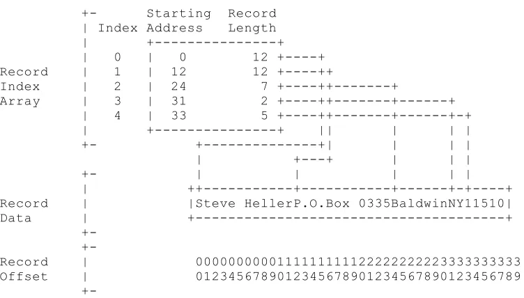
To begin, let us assume that we can describe each item by the information in the structure definition in Figure initstruct.
Item information (Figure initstruct)
typedef struct {
char upc[10];
char description[21];
float price;
} ItemRecord;
To answer this question, we have to analyze the algorithm of the binary search in some detail. We start the search by looking at the middle record in the file. If the key we are looking for is greater than the key of the middle record, we know that the record we are looking for must be in the second half of the file (if it is in the file at all). Likewise, if our key is less than the one in the middle record, the record we are looking for must be in the first half of the file (again, if it is there at all). Once we have decided which half of the file to examine next, we look at the middle record in that half and proceed exactly as we did previously. Eventually, either we will find the record we are looking for or we will discover that we can no longer divide the
segment we are looking at, as it has only one record (in which case the record we are looking for is not there).
Probably the easiest way to figure out the average number of accesses that would be required to find a record in the file is to start from the other end of the problem: how many records could be found with one access? Obviously, only the middle record. With another access, we could find either the record in the middle of the first half of the file or the record in the middle of the second half. The next access adds another four records, in the centers of the first, second, third, and fourth quarters of the file. In other words, each added access doubles the number of added records that we can find.
Binary search statistics (Figure binary.search)
Number of Number of Total accesses Total
accesses newly accessible to find all records
records records accessible
1 x 1 1 1
2 x 2 4 3
3 x 4 12 7
4 x 8 32 15
5 x 16 80 31
6 x 32 192 63
7 x 64 448 127
8 x 128 1024 255
9 x 256 2304 511
10 x 512 5120 1023
11 x 1024 11264 2047
12 x 2048 24576 4095
13 x 4096 53248 8191
14 x 1809 25326 10000
______ ______
10000 123631
Average number of accesses per record = 12.3631 accesses/record
Figure binary.search shows the calculation of the average number of accesses for a 10,000 item file. Notice that each line represents twice the number of records as the one above, with the exception of line 14. The entry for that line (1809) is the number of 14-access records needed to reach the capacity of our 10,000 record file. As you can see, the average number of accesses is approximately 12.4 per record. Therefore, at a typical hard disk speed of 10 milliseconds per access, we would need almost 125 milliseconds to look up an average record using a binary search. While this lookup time might not seem excessive, remember that a number of checkout terminals would probably be attempting to access the database at the same time, and the waiting time could become noticeable. We might also be concerned about the amount of wear on the disk mechanism that would result from this approach.
Some Random Musings
Before we try to optimize our search, let us define some terms. There are two basic categories of storage devices, distinguished by the access they allow to individual records. The first type is sequential access;1 in order to read record 1000 from a sequential device, we must read records 1 through 999 first, or at least skip over them. The second type is direct access; on a direct access device, we can read record 1000 without going past all of the previous records. However, only some direct access devices allow nonsequential accesses without a significant time penalty; these are called random access devices. Unfortunately, disk drives are direct access devices, but not random access ones. The amount of time it takes to get to a particular data record depends on how close the read/write head is to the desired position; in fact, sequential reading of data may be more than ten times as fast as random access.
Hashing It Out
Let's start by considering a linear or sequential search. That is, we start at the beginning of the file and read each record in the file until we find the one we want (because its key is the same as the key we are looking for). If we get to the end of the file without finding a record with the key we are looking for, the record isn't in the file. This is certainly a simple method, and indeed is perfectly acceptable for a very small file, but it has one major drawback: the average time it takes to find a given record increases every time we add another record. If the file gets twice as big, it takes twice as long to find a record, on the average. So this seems useless.
Divide and Conquer
But what if, instead of having one big file, we had many little files, each with only a few records in it? Of course, we would need to know which of the little files to look in, or we wouldn't have gained anything. Is there any way to know that?
Let's see if we can find a way. Suppose that we have 1000 records to search through, keyed by telephone number. To speed up the lookup, we have divided the records into 100 subfiles, averaging 10 numbers each. We can use the last two digits of the telephone number to decide which subfile to look in (or to put a new record in), and then we have to search through only the records in that subfile. If we get to the end of the subfile without finding the record we are looking for, it's not in the file. That's the basic idea of hash coding.
But why did we use the last two digits, rather than the first two? Because they will probably be more evenly distributed than the first two digits. Most of the telephone numbers on your list probably fall within a few telephone exchanges near where you live (or work). For example, suppose my local telephone book contained a lot of 758 and 985 numbers and very few numbers from other exchanges. Therefore, if I were to use the first two digits for this hash coding scheme, I would end up with two big subfiles (numbers 75 and 98) and 98 smaller ones, thus negating most of the benefit of dividing the file. You see, even though the average subfile size would still be 10, about 90% of the records would be in the two big subfiles, which would have perhaps 450 records each. Therefore, the average search for 90% of the records would require reading 225 records, rather than the five we were planning on. That is why it is so important to get a reasonably even distribution of the data records in a hash-coded file.
Unite and Rule
It is inconvenient to have 100 little files lying around, and the time required to open and close each one as we need it makes this implementation inefficient. But there's no reason we
couldn't combine all of these little files into one big one and use the hash code to tell us where we should start looking in the big file. That is, if we have a capacity of 1000 records, we could use the last two digits of the telephone number to tell us which "subfile" we need of the 100 "subfiles" in the big file (records 0-9, 10-19 ... 980-989, 990-999). To help visualize this, let's look at a smaller example: 10 subfiles having a capacity of four telephone numbers each and a hash code consisting of just the last digit of the telephone number (Figure initfile).
hash code consisting of just the last digit of the telephone number (Figure initfile).
Hashing with subfiles, initialized file (Figure initfile)
Subfile #
+---+---+---+---+ 0 | I 0000000 | I 0000000 | I 0000000 | I 0000000 | +---+---+---+---+ 1 | I 0000000 | I 0000000 | I 0000000 | I 0000000 | +---+---+---+---+ 2 | I 0000000 | I 0000000 | I 0000000 | I 0000000 | +---+---+---+---+ 3 | I 0000000 | I 0000000 | I 0000000 | I 0000000 | +---+---+---+---+ 4 | I 0000000 | I 0000000 | I 0000000 | I 0000000 | +---+---+---+---+ 5 | I 0000000 | I 0000000 | I 0000000 | I 0000000 | +---+---+---+---+ 6 | I 0000000 | I 0000000 | I 0000000 | I 0000000 | +---+---+---+---+ 7 | I 0000000 | I 0000000 | I 0000000 | I 0000000 | +---+---+---+---+ 8 | I 0000000 | I 0000000 | I 0000000 | I 0000000 | +---+---+---+---+ 9 | I 0000000 | I 0000000 | I 0000000 | I 0000000 | +---+---+---+---+
In order to use a big file rather than a number of small ones, we have to make some changes to our algorithm. When using many small files, we had the end-of-file indicator to tell us where to add records and where to stop looking for a record; with one big file subdivided into small subfiles, we have to find another way to handle these tasks.
Knowing When to Stop
One way is to add a "valid-data" flag to every entry in the file, which is initialized to "I" (for invalid) in the entries in Figure initfile, and set each entry to "valid" (indicated by a "V" in that same position) as we store data in it. Then if we get to an invalid record while looking up a record in the file, we know that we are at the end of the subfile and therefore the record is not in the file (Figure distinct).
Hashing with distinct subfiles (Figure distinct)
Subfile #
3 | I 0000000 | I 0000000 | I 0000000 | I 0000000 | +---+---+---+---+ 4 | I 0000000 | I 0000000 | I 0000000 | I 0000000 | +---+---+---+---+ 5 | I 0000000 | I 0000000 | I 0000000 | I 0000000 | +---+---+---+---+ 6 | I 0000000 | I 0000000 | I 0000000 | I 0000000 | +---+---+---+---+ 7 | I 0000000 | I 0000000 | I 0000000 | I 0000000 | +---+---+---+---+ 8 | I 0000000 | I 0000000 | I 0000000 | I 0000000 | +---+---+---+---+ 9 | I 0000000 | I 0000000 | I 0000000 | I 0000000 | +---+---+---+---+
For example, if we are looking for the number "9898981", we start at the beginning of subfile 1 in Figure distinct (because the number ends in 1), and examine each record from there on. The first two entries have the numbers "9876541" and "2323231", which don't match, so we continue with the third one, which is the one we are looking for. But what if we were looking for "9898971"? Then we would go through the first three entries without finding a match. The fourth entry is "I 0000000", which is an invalid entry. This is the marker for the end of this subfile, so we know the number we are looking for isn't in the file.
Now let's add another record to the file with the phone number "1212121". As before, we start at the beginning of subfile 1, since the number ends in 1. Although the first three records are already in use, the fourth (and last) record in the subfile is available, so we store our new record there, resulting in the situation in Figure merged.
Hashing with merged subfiles (Figure merged)
Subfile #
+---+---+---+---+ 0 | I 0000000 | I 0000000 | I 0000000 | I 0000000 | +---+---+---+---+ 1 | V 9876541 | V 2323231 | V 9898981 | V 1212121 | +---+---+---+---+ 2 | V 2345432 | I 0000000 | I 0000000 | I 0000000 | +---+---+---+---+ 3 | I 0000000 | I 0000000 | I 0000000 | I 0000000 | +---+---+---+---+ 4 | I 0000000 | I 0000000 | I 0000000 | I 0000000 | +---+---+---+---+ 5 | I 0000000 | I 0000000 | I 0000000 | I 0000000 | +---+---+---+---+ 6 | I 0000000 | I 0000000 | I 0000000 | I 0000000 | +---+---+---+---+ 7 | I 0000000 | I 0000000 | I 0000000 | I 0000000 | +---+---+---+---+ 8 | I 0000000 | I 0000000 | I 0000000 | I 0000000 | +---+---+---+---+ 9 | I 0000000 | I 0000000 | I 0000000 | I 0000000 | +---+---+---+---+
However, what happens if we look for "9898971" in the above situation? We start out the same way, looking at records with phone numbers "9876541", "2323231", "9898981", and "1212121". But we haven't gotten to an invalid record yet. Can we stop before we get to the first record of the next subfile?
Handling Subfile Overflow
To answer that question, we have to see what would happen if we had added another record that belonged in subfile 1. There are a number of possible ways to handle this situation, but most of them are appropriate only for memory-resident files. As I mentioned above, reading the next record in a disk file is much faster than reading a record at a different place in the file. Therefore, for disk-based data, the most efficient place to put "overflow" records is in the next open place in the file, which means that adding a record with phone number "1234321" to this file would result in the arrangement in Figure overflow.2
Hashing with overflow between subfiles (Figure overflow)
Subfile #
+---+---+---+---+ 0 | I 0000000 | I 0000000 | I 0000000 | I 0000000 | +---+---+---+---+ 1 | V 9876541 | V 2323231 | V 9898981 | V 1212121 | +---+---+---+---+ 2 | V 2345432 | V 1234321 | I 0000000 | I 0000000 | +---+---+---+---+ 3 | I 0000000 | I 0000000 | I 0000000 | I 0000000 | +---+---+---+---+ 4 | I 0000000 | I 0000000 | I 0000000 | I 0000000 | +---+---+---+---+ 5 | I 0000000 | I 0000000 | I 0000000 | I 0000000 | +---+---+---+---+ 6 | I 0000000 | I 0000000 | I 0000000 | I 0000000 | +---+---+---+---+ 7 | I 0000000 | I 0000000 | I 0000000 | I 0000000 | +---+---+---+---+ 8 | I 0000000 | I 0000000 | I 0000000 | I 0000000 | +---+---+---+---+ 9 | I 0000000 | I 0000000 | I 0000000 | I 0000000 | +---+---+---+---+
Some Drawbacks of Hashing
This points out one of the drawbacks of standard disk-based hashing (SDBH). We cannot delete a record from the file simply by setting the invalid flag in that record; if we did, any record which overflowed past the one we deleted would become inaccessible, as we would stop looking when we got to the invalid record. For this reason, invalid records must be only those that have never been used and therefore can serve as "end-of-subfile" markers.
While we're on the topic of drawbacks of SDBH, we ought to note that as the file gets filled up, the maximum length of a search increases, especially an unsuccessful search. That is because adding a record to the end of a subfile that has only one invalid entry left results in "merging" that subfile and the next one, so that searches for entries in the first subfile have to continue to the next one. In our example, when we added "1212121" to the file, the maximum length of a search for an entry in subfile 1 increased from four to seven, even though we had added only one record. With a reasonably even distribution of hash codes (which we don't have in our example), this problem is usually not serious until the file gets to be about 80% full.
While this problem would be alleviated by increasing the capacity of the file as items are added, unfortunately SDBH does not allow such incremental expansion, since there would be no way to use the extra space; the subfile starting positions can't be changed after we start writing records, or we won't be able to find records we have already stored. Of course, one way to overcome this problem is to create a new file with larger (or more) subfiles, read each record from the old file and write it to the new one. What we will do in our example is simply to make the file 25% bigger than needed to contain the records we are planning to store, which means the file won't get more than 80% full.
Another problem with SDBH methods is that they are not well suited to storage of variable-length records; the address calculation used to find a "slot" for a record relies on the fact that the records are of fixed length.
Finally, there's the ever-present problem of coming up with a good hash code. Unfortunately, unless we know the characteristics of the input data precisely, it's theoretically possible that all of the records will generate the same hash code, thus negating all of the performance
advantages of hashing. Although this is unlikely, it makes SDBH an inappropriate algorithm for use in situations where a maximum time limit on access must be maintained.
When considering these less-than-ideal characteristics, we should remember that other search methods have their own disadvantages, particularly in speed of lookup. All in all, the
disadvantages of such a simply implemented access method seem rather minor in comparison with its benefits, at least for the current application. In addition, recent innovations in hashing have made it possible to improve the flexibility of SDBH methods by fairly simple changes. For example, the use of "last-come, first-served" hashing, which stores a newly added record exactly where the hash code indicates, greatly reduces the maximum time needed to find any record; it also makes it possible to determine for any given file what that maximum is, thus removing one of the barriers to using SDBH in a time-critical application.3 Even more recently, a spectacular advance in the state of the art has made it possible to increase the file capacity incrementally, as well as to delete records efficiently. Chapter dynhash.htm provides a C++ implementation of this remarkable innovation in hashing.
Caching out Our Winnings
Of course, even one random disk access takes a significant amount of time, from the computer's point of view. Wouldn't it be better to avoid accessing the disk at all?
While that would result in the fastest possible lookup, it would require us to have the entire database in memory, which is usually not feasible. However, if we had some of the database in memory, perhaps we could eliminate some of the disk accesses.
A cache is a portion of a large database that we want to access, kept in a type of storage that can be accessed more rapidly than the type used to store the whole database. For example, if your system has an optical disk which is considerably slower than its hard disk, a portion of the database contained on the optical disk may be kept on the hard disk. Why don't we just use the hard disk for the whole database? The optical disk may be cheaper per megabyte or may have more capacity, or the removability and long projected life span of the optical diskettes may be the major reason. Of course, our example of a cache uses memory to hold a portion of the database that is stored on the hard disk, but the principle is the same: memory is more expensive than disk storage, and with certain computers, it may not be possible to install enough memory to hold a copy of the entire database even if price were no object.
If a few items account for most of the transactions, the use of a cache speeds up access to those items, since they are likely to be among the most recently used records. This means that if we keep a number of the most recently accessed records in memory, we can reduce the number of disk accesses significantly. However, we have to have a way to locate items in the cache quickly: this problem is very similar to a hash-coded file lookup, except that we have more freedom in deciding how to handle overflows, where the entry we wish to use is already being used by another item. Since the cache is only a copy of data that is also stored
elsewhere, we don't have to be so concerned about what happens to overflowing entries; we can discard them if we wish to, since we can always get fresh copies from the disk.
The simplest caching lookup algorithm is a direct-mapped cache. That means each key corresponds to one and only one entry in the cache. In other words, overflow is handled by overwriting the previous record in that space with the new entry. The trouble with this method is that if two (or more) commonly used records happen to map to the same cache entry, only one of them can be in the cache at one time. This requires us to go back to the disk repeatedly for these conflicting records. The solution to this problem is to use a multiway associative cache. In this algorithm, each key corresponds to a cache line, which contains more than one entry. In our example, it contains eight entries. Therefore, if a number of our records have keys that map to the same line, up to eight of them can reside in the cache simultaneously. How did I decide on an eight-way associative cache? By trying various cache sizes until I found the one that yielded the greatest performance.
the database (Figure supinit.00), and a third called supert.cpp to read the test keys and look them up (Figure supert.00). The results of this simulation indicated that, using an eight-way associative cache, approximately 44% of the disk accesses that would be needed in a noncached system could be eliminated.
Test program for caching (superm\stestgen.cpp) (Figure stestgen.00)
codelist/stestgen.00
Database initialization program for caching (superm\supinit.cpp) (Figure supinit.00)
codelist/supinit.00
Retrieval program for caching (superm\supert.cpp) (Figure supert.00)
codelist/supert.00
Figure line.size shows the results of my experimentation with various line sizes.
Line size effects (Figure line.size)
Line size Hit ratio
1 .344
2 .38
4 .42
8 .44
16 .43
The line size is defined by the constant MAPPING_FACTOR in superm.h (Figure superm.00a).
Header file for supermarket lookup system (superm\superm.h) (Figure superm.00a)
codelist/superm.00a
Now that we have added a cache to our optimization arsenal, only three more changes are necessary to reach the final lookup algorithm that we will implement. The first is to shrink each of the subfiles to one entry. That is, we will calculate a record address rather than a subfile address when we start trying to add or look up a record. This tends to reduce the length of the search needed to find a given record, as each record (on average) will have a different starting position, rather than a number of records having the same starting position, as is the case with longer subfiles.
The second change is that, rather than having a separate flag to indicate whether a record position in the file is in use, we will create an "impossible" key value to mean that the record is available. Since our key will consist only of decimal digits (compressed to two digits per byte), we can set the first digit to 0xf (the hex representation for 15), which cannot occur in a genuine decimal number. This will take the place of our "invalid" flag, without requiring extra storage in the record.
Finally, we have to deal with the possibility that the search for a record will encounter the end of the file, because the last position in the file is occupied by another record. In this case, we will wrap around to the beginning of the file and keep looking. In other words, position 0 in the file will be considered to follow immediately after the last position in the file.
Saving Storage
Now that we have decided on our lookup algorithm, we can shift our attention to reducing the amount of storage required for each record in our supermarket price lookup program. Without any special encoding, the disk storage requirements for one record would be 35 bytes (10 for the UPC, 21 for the description, and 4 for the price). For a file of 10,000 items, this would require 350 Kbytes; allowing 25% extra space to prevent the hashing from getting too slow means that the file would end up taking up about 437 Kbytes. For this application, disk storage space would not be a problem; however, the techniques we will use to reduce the file size are useful in many other applications as well. Also, searching a smaller file is likely to be faster, because the heads have to move a shorter distance on the average to get to the record where we are going to start our search.
The Code
Now that we have covered the optimizations that we will use in our price lookup system, it's time to go through the code that implements these algorithms. This specific implementation is set up to handle a maximum of FILE_CAPACITY items, defined in superm.h (Figure
superm.00a).5 Each of these items, as defined in the ItemRecord structure in the same file, has a price, a description, and a key, which is the UPC code. The key would be read in by a bar-code scanner in a real system, although our test program will read it in from the keyboard.
Some User-Defined Types
Several of the fields in the ItemRecord structure definition require some explanation, so let's take a closer look at that definition, shown in Figure superm.00.
ItemRecord struct definition (from superm\superm.h) (Figure superm.00)
codelist/superm.00
The upc field is defined as a BCD (binary-coded decimal) value of ASCII_KEY_SIZE digits (contained in BCD_KEY_SIZE bytes). The description field is defined as a Radix40 field DESCRIPTION_WORDS in size; each of these words contains three Radix40 characters.
A BCD value is stored as two digits per byte, each digit being represented by a four-bit code between 0000(0) and 1001(9). Function ascii_to_BCD in bcdconv.cpp (Figure bcdconv.00) converts a decimal number, stored as ASCII digits, to a BCD value by extracting each digit from the input argument and subtracting the code for '0' from the digit value; BCD_to_ascii (Figure bcdconv.01) does the reverse.
ASCII to BCD conversion function (from superm\bcdconv.cpp) (Figure bcdconv.00)
codelist/bcdconv.00
BCD to ASCII conversion function (from superm\bcdconv.cpp) (Figure bcdconv.01)
codelist/bcdconv.01
A UPC code is a ten-digit number between 0000000000 and 9999999999, which
unfortunately is too large to fit in a long integer of 32 bits. Of course, we could store it in ASCII, but that would require 10 bytes per UPC code. So BCD representation saves five bytes
ASCII, but that would require 10 bytes per UPC code. So BCD representation saves five bytes per item compared to ASCII.
A Radix40 field, as mentioned above, stores three characters (from a limited set of
possibilities) in 16 bits. This algorithm (like some other data compression techniques) takes advantage of the fact that the number of bits required to store a character depends on the number of distinct characters to be represented.6 The BCD functions described above are an example of this approach. In this case, however, we need more than just the 10 digits. If our character set can be limited to 40 characters (think of a Radix40 value as a "number" in base 40), we can fit three of them in 16 bits, because 403 is less than 216.
Let's start by looking at the header file for the Radix40 conversion functions, which is shown in Figure radix40.00a.
The header file for Radix40 conversion (superm\radix40.h) (Figure radix40.00a)
codelist/radix40.00a
The legal_chars array, shown in Figure radix40.00 defines the characters that can be expressed in this implementation of Radix40.7 The variable weights contains the multipliers to be used to construct a two-byte Radix40 value from the three characters that we wish to store in it.
The legal_chars array (from superm\radix40.cpp) (Figure radix40.00)
codelist/radix40.00
As indicated in the comment at the beginning of the ascii_to_radix40 function (Figure
radix40.01), the job of that function is to convert a null-terminated ASCII character string to Radix40 representation. After some initialization and error checking, the main loop begins by incrementing the index to the current word being constructed, after every third character is translated. It then translates the current ASCII character by indexing into the lookup_chars array, which is shown in Figure radix40.02. Any character that translates to a value with its high bit set is an illegal character and is converted to a hyphen; the result flag is changed to S_ILLEGAL if this occurs.
The ascii_to_radix40 function (from superm\radix40.cpp) (Figure radix40.01)
codelist/radix40.01
The lookup_chars array (from superm\radix40.cpp) (Figure radix40.02)
In the line radix40_data[current_word_index] += weights[cycle] * j;, the character is added into the current output word after being multiplied by the power of 40 that is
appropriate to its position. The first character in a word is represented by its position in the legal_chars string. The second character is represented by 40 times that value and the third by 1600 times that value, as you would expect for a base-40 number.
The complementary function radix40_to_ascii (Figure radix40.03) decodes each character unambiguously. First, the current character is extracted from the current word by dividing by the weight appropriate to its position; then the current word is updated so the next character can be extracted. Finally, the ASCII value of the character is looked up in the legal_chars array.
The radix40_to_ascii function (from superm\radix40.cpp) (Figure radix40.03)
codelist/radix40.03
Preparing to Access the Price File
Now that we have examined the user-defined types used in the ItemRecord structure, we can go on to the PriceFile structure, which is used to keep track of the data for a particular price file.8 The best way to learn about this structure is to follow the program as it creates,
initializes, and uses it. The function main, which is shown in Figure superm.01, after checking that it was called with the correct number of arguments, calls the initialize_price_file function (Figure suplook.00) to set up the PriceFile structure.
The main function (from superm\superm.cpp) (Figure superm.01)
codelist/superm.01
The initialize_price_file function (from superm\suplook.cpp) (Figure suplook.00)
codelist/suplook.00
The initialize_price_file function allocates storage for and initializes the PriceFile structure, which is used to control access to the price file. This structure contains pointers to the file, to the array of cached records that we have in memory, and to the array of record numbers of those cached records. As we discussed earlier, the use of a cache can reduce the amount of time spent reading records from the disk by maintaining copies of a number of those records in memory, in the hope that they will be needed again. Of course, we have to keep track of which records we have cached, so that we can tell whether we have to read a particular record from the disk or can retrieve a copy of it from the cache instead.
When execution starts, we don't have any records cached; therefore, we initialize each entry in these arrays to an "invalid" state (the key is set to INVALID_BCD_VALUE). If file_mode is set to
these arrays to an "invalid" state (the key is set to INVALID_BCD_VALUE). If file_mode is set to CLEAR_FILE, we write such an "invalid" record to every position in the price file as well, so that any old data left over from a previous run is erased.
Now that access to the price file has been set up, we can call the process function (Figure
superm.02). This function allows us to enter items and/or look up their prices and descriptions, depending on mode.
The process function (from superm\superm.cpp) (Figure superm.02)
codelist/superm.02
First, let's look at entering a new item (INPUT_MODE). We must get the UPC code, the description, and the price of the item. The UPC code is converted to BCD, the description to Radix40, and the price to unsigned. Then we call write_record (Figure suplook.01) to add the record to the file.
The write_record function (from superm\suplook.cpp) (Figure suplook.01)
codelist/suplook.01
In order to write a record to the file, write_record calls lookup_record_number (Figure
suplook.02) to determine where the record should be stored so that we can retrieve it quickly later. The lookup_record_number function does almost the same thing as lookup_record (Figure suplook.03), except tha the latter returns a pointer to the record rather than its number. Therefore, they are implemented as calls to a common function: lookup_record_and_number (Figure suplook.04).
The lookup_record_number function (from superm\suplook.cpp) (Figure suplook.02)
codelist/suplook.02
The lookup_record function (from superm\suplook.cpp) (Figure suplook.03)
codelist/suplook.03
The lookup_record_and_number function (from superm\suplook.cpp) (Figure suplook.04)
codelist/suplook.04
After a bit of setup code, lookup_record_and_number determines whether the record we want is already in the cache, in which case we don't have to search the file for it. To do this, we call compute_cache_hash (Figure suplook.05), which in turn calls compute_hash (Figure
suplook.06) to do most of the work of calculating the hash code.
The compute_cache_hash function (from superm\suplook.cpp) (Figure suplook.05)
codelist/suplook.05
The compute_hash function (from superm\suplook.cpp) (Figure suplook.06)
codelist/suplook.06
This may look mysterious, but it's actually pretty simple. After clearing the hash code we are going to calculate, it enters a loop that first shifts the old hash code one (decimal) place to the left, end around, then adds the low four bits of the next character from the key to the result. When it finishes this loop, it returns to the caller, in this case compute_cache_hash. How did I come up with this algorithm?
Making a Hash of Things
Well, as you will recall from our example of looking up a telephone number, the idea of a hash code is to make the most of variations in the input data, so that there will be a wide
distribution of "starting places" for the records in the file. If all the input values produced the same hash code, we would end up with a linear search again, which would be terribly slow. In this case, our key is a UPC code, which is composed of decimal digits. If each of those digits contributes equally to the hash code, we should be able to produce a fairly even distribution of hash codes, which are the starting points for searching through the file for each record. As we noted earlier, this is one of the main drawbacks of hashing: the difficulty of coming up with a good hashing algorithm. After analyzing the nature of the data, you may have to try a few different algorithms with some test data, until you get a good distribution of hash codes. However, the effort is usually worthwhile, since you can often achieve an average of slightly over one disk access per lookup (assuming that several records fit in one physical disk record).
Meanwhile, back at compute_cache_hash, we convert the result of compute_hash, which is an unsigned value, into an index into the cache. This is then returned to
lookup_record_and_number as the starting cache index. As mentioned above, we are using an eight-way associative cache, in which each key can be stored in any of eight entries in a cache line. This means that we need to know where the line starts, which is computed by
compute_starting_cache_hash (Figure suplook.07) and where it ends, which is computed by compute_ending_cache_hash (Figure suplook.08).9
The compute_starting_cache_hash function (from superm\suplook.cpp) (Figure
suplook.07)
codelist/suplook.07
The compute_ending_cache_hash function (from superm\suplook.cpp) (Figure
suplook.08)
codelist/suplook.08
After determining the starting and ending positions where the key might be found in the cache, we compare the key in each entry to the key that we are looking for, and if they are equal, we have found the record in the cache. In this event, we set the value of the record_number argument to the file record number for this cache entry, and return with the status set to FOUND.
Otherwise, the record isn't in the cache, so we will have to look for it in the file; if we find it, we will need a place to store it in the cache. So we pick a "random" entry in the line
(cache_replace_index) by calculating the remainder after dividing the number of accesses we have made by the MAPPING_FACTOR. This will generate an entry index between 0 and the highest entry number, cycling through all the possibilities on each successive access, thus not favoring a particular entry number.
However, if the line has an invalid entry (where the key is INVALID_BCD_VALUE), we should use that one, rather than throwing out a real record that might be needed later. Therefore, we search the line for such an empty entry, and if we are successful, we set
cache_replace_index to its index.
Next, we calculate the place to start looking in the file, via compute_file_hash, (Figure
suplook.09), which is very similar to compute_cache_hash except that it uses the FILE_SIZE constant in superm.h (Figure superm.00a) to calculate the index rather than the CACHE_SIZE constant, as we want a starting index in the file rather than in the cache.
The compute_file_hash function (from superm\suplook.cpp) (Figure suplook.09)
codelist/suplook.09
As we noted above, this is another of the few drawbacks of this hashing method: the size of the file must be decided in advance, rather than being adjustable as data is entered. The reason is that to find a record in the file, we must be able to calculate its approximate position in the file in the same manner as it was calculated when the record was stored. The calculation of the hash code is designed to distribute the records evenly throughout a file of known size; if we changed the size of the file, we wouldn't be able to find records previously stored. Of course, different files can have different sizes, as long as we know the size of the file we are operating on currently: the size doesn't have to be an actual constant as it is in our example, but it does have to be known in advance for each file.
Now we're ready to start looking for our record in the file at the position specified by starting_file_index. Therefore, we enter a loop that searches from this starting position toward the end of the file, looking for a record with the correct key. First we set the file pointer to the first position to be read, using position_record (Figure suplook.10), then read the record at that position.
The position_record function (from superm\suplook.cpp) (Figure suplook.10)
codelist/suplook.10
If the key in that record is the one we are looking for, our search is successful. On the other hand, if the record is invalid, then the record we are looking for is not in the file; when we add records to the file, we start at the position given by starting_file_index and store our new record in the first invalid record we find.10 Therefore, no record can overflow past an invalid record, as the invalid record would have been used to store the overflow record.
In either of these cases, we are through with the search, so we break out of the loop. On the other hand, if the entry is neither invalid nor the record we are looking for, we keep looking through the file until either we have found the record we want, we discover that it isn't in the file by encountering an invalid record, or we run off the end of the file. In the last case we start over at the beginning of the file.
If we have found the record, we copy it to the cache entry we've previously selected and copy its record number into the list of record numbers in the cache so that we'll know which record we have stored in that cache position. Then we return to the calling function, write_record, with the record we have found. If we have determined that the record is not in the file, then we obviously can't read it into the cache, but we do want to keep track of the record number where we stopped, since that is the record number that will be used for the record if we write it to the file.
To clarify this whole process, let's make a file with room for only nine records by changing FILE_SIZE to 6 in superm.h (Figure superm.00a). After adding a few records, a dump looks like Figure initcondition.
Initial condition (Figure initcondition)
Position Key Data
0. INVALID
1. INVALID
2. 0000098765: MINESTRONE:245
3. 0000121212: OATMEAL, 1 LB.:300
4. INVALID
5. INVALID
6. 0000012345: JELLY BEANS:150
7. INVALID
8. 0000099887: POPCORN:99
Let's add a record with the key "23232" to the file. Its hash code turns out to be 3, so we look at position 3 in the file. That position is occupied by a record with key "121212", so we can't store our new record there. The next position we examine, number 4, is invalid, so we know that the record we are planning to add is not in the file. (Note that this is the exact sequence we follow to look up a record in the file as well). We use this position to hold our new record. The file now looks like Figure aftermilk.
After adding "milk" record (Figure aftermilk)
Position Key Data
0. INVALID
1. INVALID
2. 0000098765: MINESTRONE:245
3. 0000121212: OATMEAL, 1 LB.:300
4. 0000023232: MILK:128
5. INVALID
6. 0000012345: JELLY BEANS:150
7. INVALID
8. 0000099887: POPCORN:99
Looking up our newly added record follows the same algorithm. The hash code is still 3, so we examine position 3, which has the key "121212". That's not the desired record, and it's not invalid, so we continue. Position 4 does match, so we have found our record. Now let's try to find some records that aren't in the file.
Wrapping Around at End-of-File
In order to continue looking for this record, we must start over at the beginning of the file. That is, position 0 is the next logical position after the last one in the file. As it happens, position 0 contains an invalid record, so we know that the record we want isn't in the file.11 In any event, we are now finished with lookup_record_and_number. Therefore, we return to lookup_record_number, which returns the record number to be used to write_record (Figure
suplook.01), along with a status value of FILE_FULL, FOUND, or NOT_IN_FILE (which is the status we want). FILE_FULL is an error, as we cannot add a record to a file that has reached its capacity. So is FOUND, in this situation, as we are trying to add a new record, not find one that alreadys exists. In either of these cases, we simply return the status to the calling function, process, (Figure superm.02), which gives an appropriate error message and continues execution.
However, if the status is NOT_IN_FILE, write_record continues by positioning the file to the record number returned by lookup_record_number, writing the record to the file, and returns the status NOT_IN_FILE to process, which continues execution normally.
That concludes our examination of the input mode in process. The lookup mode is very similar, except that it uses the lookup_record function (Figure suplook.03) rather than lookup_record_number, since it wants the record to be returned, not just the record number. The lookup mode, of course, also differs from the entry mode in that it expects the record to be in the file, and displays the record data when found.
After process terminates when the user enters "*" instead of a code number to be looked up or entered, main finishes up by calling terminate_price_file (Figure suplook.11) , which closes the price file and returns. All processing complete, main exits to the operating system.
The terminate_price_file function (from superm\suplook.cpp) (Figure suplook.11)
codelist/suplook.11
Summary
In this chapter, we have covered ways to save storage by using a restricted character set and to gain rapid access to data by an exact key, using hash coding and caching. In the next chapter we will see how to use bitmaps and distribution sorting to aid in rearranging information by criteria that can be specified at run-time.
1. What modifications to the program would be needed to support: 1. Deleting records?
2. Handling a file that becomes full, as an off-line process? 3. Keeping track of the inventory of each item?
2. How could hash coding be applied to tables in memory?
3. How could caching be applied to reduce the time needed to look up an entry in a table in memory?
(You can find suggested approaches to problems in Chapter artopt.htm).
Footnotes
1. Tape drives are the most commonly used sequential access devices.
2. In general, the "next open place" is not a very good place to put an overflow record if the hash table is kept in memory rather than on the disk; the added records "clog" the table, leading to slower access times. A linked list approach is much better for tables that are actually memory resident. Warning: this does not apply to tables in virtual memory, where linked lists provide very poor performance. For more discussion on overflow handling, see the dynamic hashing algorithm in Chapter dynhash.htm.
3. For a description of "last-come, first-served" hashing, see Patricio V. Poblete and J. Ian Munro, "Last-Come-First-Served Hashing", in Journal of Algorithms 10, 228-248, or my article "Galloping Algorithms", in Windows Tech Journal, 2(February 1993), 40-43. 4. This is a direct-mapped cache.
5. Increasing the maximum number of records in the file by increasing FILE_CAPACITY would also increase the amount of memory required for the cache unless we reduced the cache size as a fraction of the file size by reducing the value .20 in the calculation of APPROXIMATE_CACHE_SIZE.
6. The arithmetic coding data compression algorithm covered in Chapter compress.htm, however, does not restrict the characters that can be represented; rather, it takes advantage of the differing probabilities of encountering each character in a given situation.
7. Note that this legal_chars array must be kept in synchronization with the lookup_chars array, shown in Figure radix40.02.
8. While we could theoretically have more than one of these files active at a time, our example program uses only one such file.
9. This function actually returns one more than the index to the last entry in the line because the standard C loop control goes from the first value up to one less than the ending value.
10. Of course, we might also find a record with the same key as the one we are trying to add, but this is an error condition, since keys must be unique.
A Mailing List System
Introduction
In this chapter we will use a selective mailing list system to illustrate rapid access to and rearrangement of information selected by criteria specified at run time. Our example will allow us to select certain customers of a mail-order business whose total purchases this year have been within a particular range and whose last order was within a certain time period. This would be very useful for a retailer who wants to send coupons to lure back the (possibly lost) customers who have spent more than $100 this year but who haven't been in for 30 days. The labels for the letters should be produced in ZIP code order, to take advantage of the discount for presorted mail.
Algorithms Discussed
The Distribution Counting Sort, Bitmaps
A First Approach
To begin, let us assume that the information we have about each customer can be described by the structure definition in Figure custinfo.
Customer information (Figure custinfo)
typedef struct
{
char last_name[LAST_NAME_LENGTH+1];
char first_name[FIRST_NAME_LENGTH+1];
char address1[ADDRESS1_LENGTH+1];
char address2[ADDRESS2_LENGTH+1];
char city[CITY_LENGTH+1];
char state[STATE_LENGTH+1];
char zip[ZIP_LENGTH+1];
int date_last_here;
int dollars_spent;
} DataRecord;
A straightforward approach would be to store all of this information in a disk file, with one DataRecord record for each customer. In order to construct a selective mailing list, we read through the file, testing each record to see whether it meets our criteria. We extract the sort key (ZIP code) for each record that passes the tests of amount spent and last transaction date, keeping these keys and their associated record numbers in memory. After reaching the end of the file, we sort the keys (possibly with a heapsort or Quicksort) and rearrange the record numbers according to the sort order, then reread the selected records in the order of their ZIP codes and print the address labels.
It may seem simpler just to collect records in memory as they meet our criteria. However, the memory requirements of this approach might be excessive if a large percentage of the records are selected. The customer file of a mail-order business is often fairly large, with 250000 or more 100-byte records not unheard of; in this situation a one-pass approach might require as much as 25