Full Terms & Conditions of access and use can be found at
http://www.tandfonline.com/action/journalInformation?journalCode=ubes20
Download by: [Universitas Maritim Raja Ali Haji] Date: 13 January 2016, At: 01:03
Journal of Business & Economic Statistics
ISSN: 0735-0015 (Print) 1537-2707 (Online) Journal homepage: http://www.tandfonline.com/loi/ubes20
Martingale Property of Exchange Rates and
Central Bank Interventions
Kamil Yilmaz
To cite this article: Kamil Yilmaz (2003) Martingale Property of Exchange Rates and
Central Bank Interventions, Journal of Business & Economic Statistics, 21:3, 383-395, DOI: 10.1198/073500103288619034
To link to this article: http://dx.doi.org/10.1198/073500103288619034
View supplementary material
Published online: 01 Jan 2012.
Submit your article to this journal
Article views: 57
View related articles
Martingale Property of Exchange Rates
and Central Bank Interventions
Kamil Y
ILMAZCollege of Administrative Sciences and Economics, Koç University, Rumelifeneri Yolu, Sariyer 34450, Istanbul, Turkey (kyilmaz@ku.edu.tr)
This article uses the variance ratio-based multiple comparison test and the Richardson–Smith Wald test procedures to test for the martingale property of daily exchange rates of seven major currencies vis-à-vis the U.S. dollar. To allow for the possibility that exchange rates are not governed by a single process throughout the oat, the test statistics are calculated and plotted for xed-length moving subsample win-dows rather than being applied to the full sample. The results show that exchange rates do not always follow the martingale process. During the times of coordinated central bank interventions, exchange rates deviate from the martingale property.
KEY WORDS: Fixed-length moving subsample window; Joint variance ratio test; Multiple comparison test; Richardson–Smith Wald test.
1. INTRODUCTION
Since the breakdown of the Bretton Woods system in the early 1970s, exchange rate economics has become an area of active research for economists. Earlier, the focus was more on structural models to explain exchange rate behavior over time. However, since Meese and Rogoff (1983) showed that the struc-tural models had inferior performance than a naïve martingale in out-of-sample forecasts, many studies strived to uncover the empirical regularities in exchange rate behavior.
Baillie and Bollerslev (1989) found evidence supporting the presence of cointegration among 7 major daily exchange rates during the period between 1980 and 1986. However, Diebold, Gardeazabal, and Yõlmaz (1994) showed that the results
ob-tained by Baillie and Bollerslev (1989) were sensitive to the inclusion of a drift in the tests, which happened to be in the data during the 1980–1986 period. Once the drift is included, evidence turns against the cointegration, and the random walk performs better than alternative models in out-of-sample fore-casts.
Applying the variance ratio (VR) test to weekly exchange rates between August 1974 and March 1989, Liu and He (1991) rejected the martingale hypothesis for the German mark (DEM), Japanese yen (JPY), and British pound (GBP), but failed to do so for the Canadian dollar (CD$) and French franc (FRF) vis-à-vis the U.S. dollar (US$). In a recent follow-up, Fong, Koh, and Ouliaris (1997) emphasized the shortcomings of Liu and He’s analysis. They studied the statistical perfor-mance of two different multiple VR tests of the martingale hy-pothesis: Hochberg’s (1974) multiple comparison test (MCT) and Richardson and Smith’s (1991) (RS) Wald test. Then they applied these tests to exchange rates over the October 1979– March 1989 period. They found that the RS test failed to reject the martingale hypothesis for all ve exchange rates consid-ered, whereas the MCT continued to reject the hypothesis for the FRF, DEM, and JPY.
Tests of the martingale hypothesis are related to the correlo-gram of log exchange rate increments. They evaluate whether the autocorrelation coefcients at different lags and leads equal 0. Liu and He (1991) and Fong et al. (1997), among oth-ers, conducted tests of martingale property in nancial time series for a given time period and reached a verdict about the
behavior of the asset prices during that period. However, it is not correct to assume that the process that governs the time series behavior of exchange rates stayed unchanged during a 25-year period. Central bank interventionsin the foreign exchange (FX) markets or the frequent realignments in the exchange rate mech-anism of the European monetary system (EMS) are some fac-tors that might possibly have affected the behavior of exchange rates over time. For example, Dominquez (2001) provided ev-idence that central bank interventions inuence intradaily FX returns and volatility.
Given the fact that central banks of major industrial countries have changed their stance with respect to market intervention over time, there is a possibility that policy shifts can result in a change in the time series behavior of exchange rates. For ex-ample, as Dominquez (1998) stated; after 4 years of passive intervention policy between 1981 and 1984, the Federal Re-serve became more active toward the end of 1985 to slow down the appreciation of the dollar against other major currencies. These shifts in the policy stance must be taken into account. One alternative then is to assume a priori that there is a struc-tural break in the data. For example, taking into account the changes in the Federal Reserve’s operating procedures, Liu and He (1991) treated October 1979 as a structural breakpoint and divided their sample in two. This is a step in the right direction, but it still falls short of a satisfactory solution for the problem at hand. Even if a change occurs in the time series behavior of ex-change rates, this does not have to be a signicant discrete jump in the underlying parameters. As long as the change takes the form of a slow, continous process or a small jump in the para-meters, structural break tests are unlikely to capture the change (Diebold and Chen 1996).
In this article it is suggested that tests of the martingale prop-erty in exchange rates need to control for the sensitivity of the results to the particular sample period used. For that reason, tests of the martingale property were conducted in moving-subsample windows with a xed length of 1,000 daily obser-vations. The test statistics for all subsample windows are plot-ted. Plotting the test statistics for subsample windows facilitates
© 2003 American Statistical Association Journal of Business & Economic Statistics July 2003, Vol. 21, No. 3 DOI 10.1198/073500103288619034 383
observation of whether there is any change in the behavior of exchange rates over time.
Following Fong et al. (1997), the present work uses two joint VR test procedures. These are the MCT proposed by Chow and Denning (1993) and the joint VR test developed by Richard-son and Smith (1991). These tests are applied to changes of daily New York spot exchange rates of the U.S. dollar vis-à-vis seven major currencies: the DEM, JPY, GBP, FRF, Swiss franc (CHF), CD$, and Italian lira (ITL). The sample period starts on January 1, 1974 and ends on February 12, 2001.
This article is not an attempt to develop a theory that shows how the martingale property can be rejected after the central bank interventions. However, theoretical models can be used to establish the link between the monetary policy actions and the violation of the martingale. McCallum (1994) and Mered-ith and Chinn (1998) presented theoretical models showing that the violation of the uncovered interest parity (UIP) can be due to the presence of feedback mechanisms between the exchange rates, ination, output, and interest rates. Under the assumption that the daily risk-free interest rate is 0, which is not a totally unjustied approximation with daily data, the UIP implies that the daily exchange rate is a martingale. Based on this assump-tion, it is theoretically possible for the monetary policy feed-back mechanisms to cause daily exchange rates to deviate from martingale behavior.
The article is organized as follows. Section 2 briey reviews the developments in the foreign exchange markets since the oat, as well as the literature on exchange rate behavior. Sec-tion 3 provides a detailed account of the joint VR tests used in the analysis, and Section 4 presents the empirical results. Sec-tion 5 concludes by summarizing the results.
2. EXCHANGE RATES UNDER THE FLOAT:
THE MARKET, CENTRAL BANK INTERVENTIONS, AND THE LITERATURE
2.1 Foreign Exchange Markets
Established as an informal market in the 1960s, FX markets grew rapidly in the 1980s and especially in the 1990s.
Accord-ing to surveys conducted by the Bank for International Set-tlements (BIS) every 3 years, since April 1989 average daily turnover in foreign exchange markets worldwide (adjusted for cross-border and local double-counting and evaluated at April 1998 exchange rates) increased by 33%, 29%, and 46% be-tween consecutive triennial surveys.
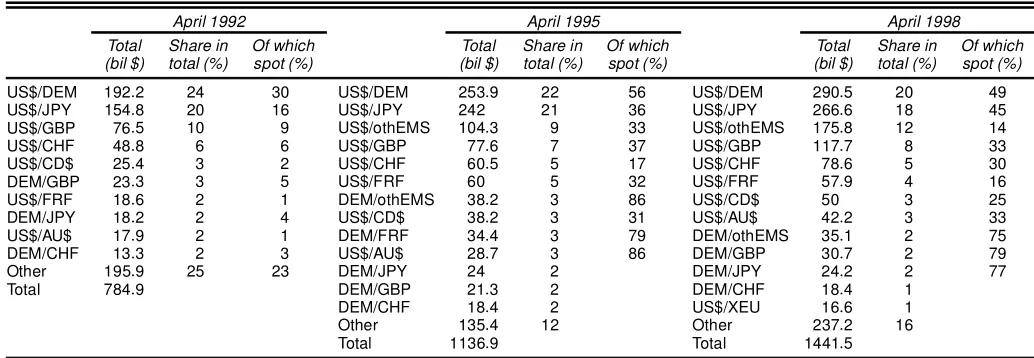
The U.S. dollar has been the dominant currency in both the spot and the forward and swap transactions. Its share in daily turnover has uctuated between 80% and 90% (when reported on one side of the transactions). The sum of the remaining six major currencies (all included in our analysis) accounts for a market share approximately equal to that of the U.S. dollar. The remaining 20%–30% of the total (200%) market turnover has been accounted by other currencies from Europe and as well as from other parts of the world (Table 1).
BIS surveys also include information on the liquidity of bilat-eral FX transactions. U.S. dollar bilatbilat-eral exchange rates against six major currencies in the sample herein form the most liquid segments of the FX market. For example, 63% of average daily trade volume in April 1998 was accounted by the bilateral U.S. dollar transactions against other major currencies included in our analysis, except ITL.
The data used in this article are reported noon spot exchange rates in New York. For that reason, it is quite relevant to study the turnover of each currency in the New York market. Table 1 reports the average daily turnover in 1995 for the seven major currencies in the New York market in their respective base mar-kets and the world market as a whole.
Based on this data, the currencies can be classied into three groups. With $104 and $55 billion daily turnovers, the DEM and JPY are the two most actively traded currencies in the New York market after the US$. Next are the three European currencies (the GBP, FRF, and CHF), each with an approxi-mate $20 billion daily turnover. Finally, the daily turnovers for the CD$ and Australian dollar (AU$) are less than $10 billion.
Table 1 reveals that spot markets went through a rapid ex-pansion in the rst half of the 1990s. Whereas on average only $140 billion worth of currency changed hands daily in 1992, according to BIS surveys this amount increased to more than
Table 1. Total Daily Turnover in FX Markets
April 1992 April 1995 April 1998
Total Share in Of which Total Share in Of which Total Share in Of which
(bil $) total (%) spot (%) (bil $) total (%) spot (%) (bil $) total (%) spot (%)
NOTE: After adjusting for double counting in interbank transactions, the average daily turnover in the New York market was 26.1 billion per day in April 1983. Other currencies in the EMS are denoted by othEMS.
Source: Bank of International Settlements (1992, 1995, 1998).
$500 billion in 1995. The expansion of the spot FX markets continued in the second half of the 1990s, although with some slowdown. Whereas total daily FX market turnover increased by 27% from 1995 to 1998, most of this increase was due to the expansion in the forward FX markets. Daily total spot market turnover increased by only 14%, to $590 billion.
Comparable gures for the 1970s and 1980s are not avail-able. However, it is evident from the available data that the FX markets have gone through a period of rapid expansion in the 1990s.
2.2 Central Bank Interventions
Especially in the earlier years of the oat, FX markets have gone through periods of instability. All major industrial coun-tries were affected adversely by oil crises in 1973 and 1979. The oil price hikes not only disturbed their external balances, but also led to high ination rates never before seen in these countries in the postwar period. The impact on the relative val-ues of major currencies was unprecedented, leading to subtan-tial volatility in the foreign exchange markets. Due to increased inationary pressures and rapid decline in the political power of the Carter administration, toward the end of the 1970s, the U.S. dollar started to lose value against other major currencies.
In the rst 2 years of the oat central banks intervened spo-radically with no coordination. The intervention was seen as a necessary policy tool to stabilize highly volatile FX markets. However, in October 1974 the U.S. Federal Reserve, the Ger-man Bundesbank, and the Swiss National Bank began interven-ing in a concerted fashion to control the volatility of the DEM and CHF exchange rates (Schwartz 2000). The coordinated in-terventions continued throughout the 1970s, with the participa-tion of the Bank of Japan after September 1977. But despite the U.S. interventions, the U.S. dollar continued to depreciate until 1980.
Differences among industrial countries’ responses to oil price shocks continued to shape the policy issues and debates in the 1980s. To bring ination under control, the Federal Reserve be-gan to follow a tight monetary policy in 1980. The resulting high interest rates attracted capital inows to the United States, leading to the appreciation of the U.S. dollar. The appreciation of the dollar lasted until 1985, and at its peak in late Febru-ary and early March 1985, the dollar was overvalued by 40% (Obstfeld 1990).
After coming to power in 1981, the Reagan administration followed a policy of little intervention. It refused any coordi-nated intervention in FX markets except in an emergency case. The concerted interventions that occurred for a short period in June–August 1982 were consistent with this policy stance. However, faced with ever rising dollar for over 4 years, the U.S. government could not stick to its promise and had to search for coordination among major central banks.
The period 1986–1991 was a time of concerted interventions in FX markets around the world. In September 1985, G-7 -nance ministers agreed to intervene in the worldwide FX mar-kets in a concerted fashion when they nd it necessary. This agreement, known as the Plaza Accord, marked a drastic change in the policy stance of the major central banks in terms of the movements of exchange rates. Soon after the signing of the
Plaza Accord came a heavy bout of concerted interventions. Most of the interventions took the form of selling U.S. dollars against other major currencies, especially against the DEM and the JPY.
These interventions paid off; the US$ started to lose much of the value that it had gained against other currencies, thanks in large part to the massive sterilized interventions by the Fed-eral Reserve, the Bundesbank, and the Bank of Japan. These in-terventions were effective in signaling the policy stance of the monetary authorities and thus could lead to some predictable
changes in the exchange rates during the second half of 1980s (Dominquez 1990).
After the success of the Plaza Accord, leading central bankers continued to work closely to prevent wide swings in the exchange rates. The Louvre Accord of February 1987 was an explicit step in this direction. It set unannounced and secret target bands for the DEM/US$ (between 1.6 and 1.9) and the JPY/US$ (between 120 and 140) exchange rates, beyond which central banks had agreed to intervene.
According to Catte, Galli, and Rebecchini (1994), the lead-ing central banks had undertaken 17 concerted interventions between 1985 and 1991. The U.S. Federal Reserve, the Bun-desbank, and the Bank of Japan were the major players in every intervention. During this period, none of the G-3 central banks undertook any intervention contradicting the policies of the other two. McKinnon (1996, pp. 67–68) emphasized that 16 out of 17 interventions during this period could be desribed as “leaning against the wind.”
Contrary to the implications of the theory, there is consen-sus among economists on whether central bank interventions have some lasting effects on FX markets. In the absence of an explicit coordination, these interventions had to be steril-ized to keep the monetary stability intact. Baillie and Osterberg (1997) showed that in the 1980s, the effects of sterilized in-terventions lasted beyond the day of intervention. Dominquez (1990) showed that the effects of sterilized intervention dimin-ish monotonically over time, and that concerted interventions are more effective than individual interventions in generating the desired exchange rate behavior.
McKinnon (1993) claimed that these infrequently exercised, explicitly announced concerted interventions affected the FX markets, simply because they signaled the policy stance of the major central banks and, thus inuenced the expectations about the future behavior of exchange rates. Obstfeld (1990), on the other hand, claimed the contrary. Based on anecdotal evidence, he argued that sterilized interventions were effective only when backed by appropriate monetary policy adjustments. Together, these studies show that changes in FX monetary, or scal poli-cies do have some lasting impact on FX markets.
In addition to these studies, Dominquez (1998) showed that central bank interventions on average led to higher volatility in bilateral DEM/US$ and JPY/US$ exchange rates. With a value of 6.14, the maximum conditional volatility for DEM/US$ oc-curred in November 2, 1978, soon after the Carter administra-tion’s decision to intervene in markets to support a declining U.S. dollar. In the case of the JPY/US$ exchange rate, the max-imum volatility was 3.27, observed just 2 days after the Plaza Accord was signed.
Because not all of the central banks were involved in all of the concerted policy interventions, market interventions cannot
be expected to affect bilateral exchange rates of the U.S. dollar vis-à-vis all other major currencies. Being the issuers of most traded currencies, the Federal Reserve, the Bundesbank,and the Bank of Japan intervened selectively to affect the value of the US$ vis-à-vis the DEM, JPY, and, to some extent, GBP. Con-sequently, if policy interventions do have lasting impact, then these bilateral exchange rates are relatively more likely to di-verge from martingale behavior during the period of concerted policy interventions.
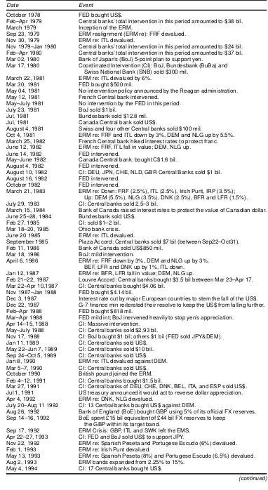
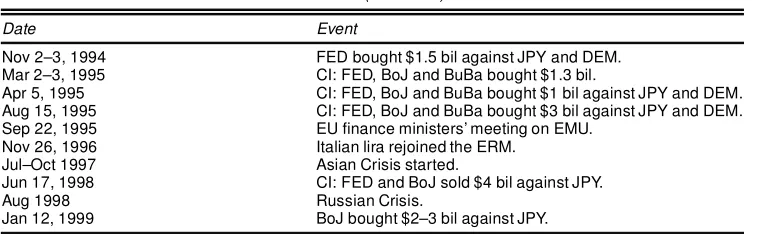
In comparison to the 1980s, throughout the 1990s fewer FX market interventions occurred. According to news reports, in-terventions of the 1990s are in general smaller in magnitude than those of the previous decade. Nine relatively small-scale interventions were undertaken between 1991 and 1999 (Ta-ble 2). One important reason behind this change was the rela-tive calm in the FX markets around the world in the 1990s. The large swings that characterized the FX markets in the 1980s, especially when the U.S. dollar was concerned, were not ob-served in the 1990s; therefore, the need for policy intervention occurred less frequently and at a smaller scale.
The only exception to the relative calm of the 1990s was the ERM crisis of September 1992. After excessive speculative at-tacks, the GBP, ITL, and the Swedish kroner dropped out of the ERM and were allowed to oat freely since then. During the ERM crisis, central banks of the respective countries in-tervened heavily to defend their ERM exchange rates. The -nancial crises in Mexico, East Asia, and Russia did not have any major impact in the worldwide FX markets for major cur-rencies and thus did not necessitate policy intervention by the central banks of the G-7 countries. Recently, calls for concerted intervention intensied after the apparent failure of the Euro to recover its losses against the U.S. dollar after the Euro’s inau-guration in January 1999.
2.3 Literature on the Martingale Property of Exchange Rates
Since the breakdown of the Bretton Woods system, numerous studies on the behavior of exchange rates under the oat have been reported. The work of Meese and Rogoff (1983) has been among the most inuential. Using short-horizon log exchange rate changes, these authors showed that the structural models of exchange rate determination (i.e., the exible-price mone-tary model, the sticky-price monemone-tary model, and the portfolio-balance model) do not perform better than the random-walk model in out-of-sample forecasts.
Using more recently developedcointegrationtest procedures, Baillie and Bollerslev (1989) found evidence supporting the presence of cointegration among seven major daily exchange rates during the period 1980–1986. A nding of cointegration would mean a long-run equilibrium relationship between ex-change rates. Short-run deviations from this long-run equilib-rium relationship (called the error-correction model) can be pre-dicted. Using a maximum likelihood–based Johansen test pro-cedure, Diebold et al. (1994) showed that the results obtained by Baillie and Bollerslev (1989) were sensitive to the inclu-sion of a drift in the tests, which happened to be in the data during the 1980–1986 period. Once the drift is included, evi-dence turns against the cointegration. Diebold et al. (1994) also
showed that the random walk performs better in out-of-sample forecasts compared with alternatives such as error-correction model that would be implied by the presence of cointegration and unrestricted vector autoregression (VAR).
Besides the studies focusing on short-horizon log exchange rate changes, a whole set of studies provides direct and indi-rect evidence against random-walk behavior at long horizons. First, a series of panel studies show that purchasing power par-ity, an alternative to random-walk behavior, holds in the long run but not in the short run (Lothian 1996, Papell 1997). Sec-ond, using long-horizon changes, Lothian and Taylor (1996) showed that the real exchange rate mean reverts and that uni-variate rst-order autoregressive models perform better than al-ternative random-walk models both before and after the oat. Third, Mark (1995), Chinn and Meese (1995), and Mark and Sul (2001) found that exchange rate deviations from monetary fundamentals predict future exchange rates. Finally, Meredith and Chinn (1998) showed that uncovered interest parity may hold over long horizons, but not over short horizons.
Without a doubt, these results provide evidence that at long horizons, exchange rates do not follow random-walk behavior. Placed against the evidence supporting random-walk behavior at short horizons, this result raises a serious question: Because the long-horizon log exchange rate change is the sum of short-horizon changes, it is surprising that there is little evidence against the random walk over short horizons. In this regard, this article should be viewed as an attempt to reconcile results of the short-horizon tests with those of the long-horizon tests.
Attempts have been made to use semiparametric procedures to test for the martingale property of exchange rates. The main problem with these tests arises if the null hypothesis is rejected, in which case there is no way to determine the alternative hy-pothesis. Liu and He (1991) applied the VR test for the martin-gale property on ve major exchange rates (DEM, JPY, GBP, CD$, and FRF) against the US$ over the sample period August 1974–March 1989. They used the VR test and rejected the mar-tingale property for the DEM, JPY, and GBP, but failed to do so for the CD$ and FRF vis-à-vis the US$ for weekly exchange rates.
Fong et al. (1997) studied the statistical performance of two different multiple VR tests of the martingale hypothesis: Hochberg’s MCT and the RS Wald test. Fong et al. (1997) took their analysis one step further and applied the multiple VR test and the RS Wald test to the same data. They started by show-ing that in small samples, the RS Wald test had better power properties than the multiple VR test. When they applied both tests to the October 1979–March 1989 period, the RS Wald test failed to reject the martingale hypothesis, whereas the multiple VR test continued to reject the hypothesis for the FRF, DEM, and JPY.
All studies testing the martingale property of exchange rates were based on a xed sample period. This sample period is dic-tated either by the availability of the data or by visible breaks, such as a switch in the monetary or exchange rate policy in the country of interest. For example, Liu and He (1991) di-vided their sample into 1974–1978 and 1979–1989 to take into account a major change in U.S. monetary policy. In their analysis of the implications of the European ERM on the ex-change rate dynamics, Anthony and MacDonald (1998) divided
Table 2. Chronology of Events Concerning the FX Markets
Date Event
October 1978 FED bought US$.
Feb–Apr 1979 Central banks’ total intervention in this period amounted to $38 bil. March 1979 Inception of the ERM.
Sep 23, 1979 ERM realignment (ERM re): FRF devalued. Nov 30, 1979 ERM re: ITL devalued.
Nov 1979–Jan 1980 Central banks’ total intervention in this period amounted to $24 bil. Feb–Apr 1980 Central banks’ total intervention in this period amounted to $37 bil. Mar 02, 1980 Bank of Japan’s (BoJ) 5-point plan to support yen.
Mar 17, 1980 Coordinated Intervention (CI): BoJ, Bundesbank (BuBa) and Swiss National Bank (SNB) sold $300 mil.
March 22, 1981 ERM re: ITL devalued by 6%. Mar 30, 1981 FED bought $500 mil.
May 04, 1981 No-intervention policy announced by the Reagan administration. May 12, 1981 French Central bank intervened.
May–July 1981 No intervention by the FED in this period. July 23, 1981 BoJ sold $1 bil.
Jul, 1981 Bundesbank sold $12.8 mil. Jul, 1981 Canada Central bank sold US$.
August 4, 1981 Swiss and four other Central banks sold $100 mil.
Oct 4, 1981 ERM re: FRF and ITL down by 3%, DEM and NLG up by 5.5%. March 25, 1982 French Central bank hiked interest rates to protect franc. June 12, 1982 ERM re: FRF, ITL fall in value; DEM, NLG up.
June 14, 1982 FED intervened.
May–June 1982 Canada Central bank: bought C$1.6 bil. August 4, 1982 FED intervened.
August 10, 1982 CI: DEU, JPN, CHE, NLD, GBR Central Banks sold $1 bil. August 16, 1982 FED intervened.
October 1982 FED intervened.
March 21, 1983 ERM re: Down: FRF (2.5%), ITL (2.5%), Irish Punt, IRP (3.5%); Up: DEM (5.5%), NLG (3.5%), DNK (2.5%), BFR and LFR (1.5%). July 29, 1983 CI: Central banks sold 2.5–3 bil.
March 15, 1984 Bank of Canada raised interest rates to protect the value of Canadian dollar. June 25–28, 1984 Bundesbank sold US$.
Feb 27, 1985 CI: sold $1–2 bil. Mar 18–20, 1985 Ohio bank crisis. June 20 1985 ERM re: ITL devalued.
September 1985 Plaza Accord: Central banks sold $7 bil (between Sep22–Oct31). Feb 11, 1986 Bank of Canada sold US$850 mil.
Mar 18, 1986 BoJ: mild intervention.
April 6, 1986 ERM re: FRF down by 3%, DEM and NLG up by 3%. BEF, LFR and DNK up by 1%, ITL down.
Jan 12, 1987 ERM re: BFR, LFR fall in value; DEM, NLG up.
Feb 21–22, 1987 Louvre Accord: Central banks bought $3.5 bil between Mar 23–Apr 17. Mar 22–Apr 10,1987 CI: Central banks bought $4.06 bil.
Nov 1987–Jan 1988 FED bought $4.14 bil.
Dec 3, 1987 Interest rate cut by major European countries to stem the fall of the US$. Dec 22, 1987 G-7 nance min reiterated their resolve to keep the US$ from falling further. Feb–Apr 1988 FED bought $818 mil.
Mar–Apr 1988 FED mild int; BoJ inervened heavily to stop yen’s appreciation. Apr 14–15, 1988 CI: Massive intervention.
May–July 1988 CI: Central banks sold $2.93 bil.
Nov 17, 1988 CI: BoJ bought $1 bil; others $1 bil (FED sold JPY&DEM). Jan 11, 1989 CI: Central banks sold US$.
May 22–Jun 7, 1989 CI: Central banks sold $10 bil. Sep 24–Oct 5, 1989 CI: Central banks sold US$. Jan 8, 1990 ERM re: ITL devalued against DEM. Mar 5–7, 1990 CI: Central banks sold US$. October 1990 British pound joined the ERM. Feb 4–12, 1991 CI: Central banks bought $1.5 bil.
Mar 27, 1991 CI: Central banks of DEU, CHE, DNK, BEL, ITA, and ESP sold US$. Jul 1, 1991 US treasury announced it would act to reverse dollar appreciation. Apr 4, 1992 ERM re: DNK, NLG devalued.
July 20–Aug 11 1992 CI: 13 Central banks bought US$ against DEM.
Aug 26, 1992 Bank of England (BoE) bought GBP using 5% of its ofcial FX reserves. Sep 14–16, 1992 BoE spent £15 bil equivalent of £44 bil FX reserves to keep
the GBP within its target band.
Sep 17, 1992 ERM Crisis: GBP, ITL and SWK left the EMS. Apr 22–27, 1993 CI: FED and BoJ sold US$ to support JPY.
Nov 22, 1992 ERM re: Spanish Peseta and Portugese Escudo (6%) devalued. Feb 1, 1993 ERM re: Irish Punt devalued.
May 13, 1993 ERM re: Spanish Peseta (8%) and Portugese Escudo (6.5%) devalued. Aug 2, 1993 ERM bands expanded from 2.25% to 15%.
May 4, 1994 CI: 17 Central banks bought US$.
(continued)
Table 2. (continued)
Date Event
Nov 2–3, 1994 FED bought $1.5 bil against JPY and DEM. Mar 2–3, 1995 CI: FED, BoJ and BuBa bought $1.3 bil.
Apr 5, 1995 CI: FED, BoJ and BuBa bought $1 bil against JPY and DEM. Aug 15, 1995 CI: FED, BoJ and BuBa bought $3 bil against JPY and DEM. Sep 22, 1995 EU nance ministers’ meeting on EMU.
Nov 26, 1996 Italian lira rejoined the ERM. Jul–Oct 1997 Asian Crisis started.
Jun 17, 1998 CI: FED and BoJ sold $4 bil against JPY. Aug 1998 Russian Crisis.
Jan 12, 1999 BoJ bought $2–3 bil against JPY.
the 1979–1992 sample into subsamples using the date of cur-rency’s realignment in the ERM as cutoff dates. Although this allowed them to clean their data from the effects of the jumps in the exchange rates during the realignment period, nevertheless in some instances they were left with few data points (fewer than 200 observations) to estimate VRs. However, both Lo and MacKinlay (1988) and Richardson and Smith (1991) showed that the VR-test has poor performance with small samples.
Moving xed-length subsample windows enables one to identify shocks that signicantly alter the exchange rate be-havior, such as the FX market interventions by central banks and the ERM realignments in the case of European currencies. These shocks on the exchange rate behavior are identied by signicant jumps in the test statistic.
3. JOINT VARIANCE RATIO TESTS
Tests of martingale hypothesis are related to the correlogram of log exchange rate increments and evaluate whether the au-tocorrelation coefcients at different lags and leads are equal to 0. Because tests of random walk do not run the risk of mis-specication of the alternative hypothesis, they are expected to be theoretically reliable. In practice, however, they have been found to have quite low statistical power. Consequently, even when a particular exchange rate follows martingale behavior, the null hypothesis can sometimes be rejected. Among the tests that rely on alternative representations of the autocorrelogram of the return series are the VR test (Cochrane 1991; Lo and MacKinlay 1988), the Fama and French (1988) regression test, and the Jegadeesh (1991) regression test.
What differentiates Lo and MacKinlay’s VR test from oth-ers [mainly from the one used by Cochrane (1991) and Poterba and Summers (1988)] is that it is possible to conduct the test even when stock returns are heteroscedastic. The VR test statis-tic is a weighted sum of estimated autocorrelation coefcients, with the weights declining in the return horizon. Being a two-tailed test, rejection by the VR test reveals information about autocorrelation structure. If the VRs at different return hori-zons are greater (smaller) than 1, then one can condently con-clude that stock returns are positively (negatively) correlated. Accordingly, a value of 1 for the VR means that stock prices follow random walk. Random-walk series have a unit root, and random-walk increments are required to be uncorrelated. Lo and MacKinlay (1988) examined the VR, Dickey–Fuller, and Box–Pierce tests and found that the VR test was more powerful than the others under the heteroscedastic random-walk model.
Lo and MacKinlay (1988) used the idea behind VRs to test for independently and identically distributed (iid) Gaussian in-crements rst, and then extended it to the case with uncorrelated but heteroscedastic increments. Lo and MacKinlay’s Monte Carlo power tabulations showed that the VR test yielded higher power under both approximations compared to the Dickey– Fullerttest and the Box–Pierce portmanteauQtest. The VR test is preferred when the focus is the absence of correlation among the increments.
Lo and MacKinlay’s VR test procedure can be applied when returns are heteroscedastic, given that they are uncorrelated with each other. If the increments are uncorrelated, then the sum of the variances of the increments should be equal to the sum of their variances, and the VR should move closer to 1 even with heteroscedastic disturbances. The asymptotic vari-ance will depend on the degree and type of heteroscedasticity present. Rather than specifying the form of heteroscedasticityin increments, Lo and MacKinlay (1988) followed White (1980) in deriving variance VRs that allow for general forms of het-eroscedasticity. They made use of the relationship between the VR and autocorrelation coefcients to derive the asymptotic distribution of the VR estimator under heteroscedastic distur-bances.
Lo and MacKinlay’s heteroscedasticity-consistent VR test statistic,z¤.q/, is used to test the null hypotheses for a spe-cic aggregation value (holding period),q. Ifz¤.q/is greater than the critical value of the standard normal distribution, then the random-walk hypothesis is rejected. However, because VRs may be statistically close to 1 for someq and different from 1 for others, the VR test procedure based on various holding periods can easily lead to inconclusive results.
Chow and Denning (1993) proposed a solution to this prob-lem. They used Hochberg’s (1974) theorem on MCTs and extended the Lo–MacKinlay VR test to incorporate multiple comparisons of selected VRs with 1. Takingk VR test sta-tistics,z¤.q
i/s, for iD1;2; : : : ;k, that have standard normal distribution under the random-walk null hypothesis, and using a Bonferroni probability inequality, the Hochberg (1974) test amounts to picking up the test statisticsz¤.q
i/with the largest absolute value. Hochberg (1974) showed that the largest ab-solute value of thesekstandard normal variates has a student-ized maximum modulus (SMM) distribution with k and nq
(sample size) degrees of freedom. The critical values for the SMM distribution are greater than the critical values for the standard normal distribution. This is not surprising given that the MCT statistic is the maximum of the VR test statistics for
all selected holding periods. The critical values of the SMM distribution were provided by Hahn and Hendrickson (1971).
The other joint VR test used in this article was developed by Richardson and Smith (1991) and makes explicit use of the serial correlation among VRs when the observations used to calculate VR overlap. If one wants to calculate the VR for a 4-day holding horizon using a sample of 100 observations, then he or she would either have 25 nonoverlappingobservations or 97 overlappingobservations for 4-day returns. Obviously, using overlapping observations will substantially increase the sample size from which to calculate VRs. However, the distribution of VRs of different return horizons calculated from overlapping data is likely to be nonnormal, because of the serial correlation among the VRs. For a given number (saym) of VRs with dif-ferent return horizons, Richardson and Smith (1991) derived a Wald test procedure to test for the null hypothesis which explic-itly takes into account the serial correlation amongmVRs.
4. TEST RESULTS: FULL-SAMPLE AND FIXED-LENGTH
MOVING-SUBSAMPLE WINDOWS
Our dataset includes daily exchange rates for January 2, 1974–February 12, 2001. The data are downloaded from the Federal Reserve Bank of Chicago’s website (http://www.frbchi. orgeconinfo/nance/for-exchange/welcome.html) and cover the period January 1971–February 2001. Because many countries switched to a oating exchange rate regime in the period 1971– 1973, following earlier literature, the sample here is restricted to the period January 1, 1974–February 12, 2001. The same tests were conducted also including the data for the 1971–1974 period, and no qualitative change was found in the results.
The analysis used daily, rather than weekly, exchange rates for two reasons. First, the literature on FX market interventions emphasizes that the effects of interventions occur immediately and diminish monotonically over time (Dominquez 1990). Us-ing weekly exchange rates would preclude capturUs-ing the imme-diate effects of the interventions. Second, unlike the case with stock returns, using daily exchange rates avoids the problem of spurious correlation caused by infrequent trading. As discussed earlier, the FX markets are very liquid. Because the tests are being applied on exchange rate returns and not on stock market index returns (which are composed of dozens of stocks, some of which may be traded infrequently), the daily exchange rates can be used without much worry.
The empirical analysis herein focuses on daily exchange rates of the US$ against seven major currencies: DEM, JPY, CHF, FRF, GBP, ITL, and CD$. Fixed-length moving windows
with 1,000 daily observations are considered. A window length of 1,000 days is chosen to ensure that the results will not suffer from small sample bias and will be comparable with the results of Liu and He (1991) and Fong et al. (1997), which had 785 observations in their samples.
The rst subsample window starts on January 2, 1974 and ends on December 29, 1977. After the joint VR test statistic for the rst subsample is calculated, the window is moved ve daily observations forward, and the joint VR test statistic is re-calculated. (It was decided to increase the sample size by ve daily observations at a time to save on computer time.) Once the test statistics for all windows are obtained, they are plotted, and their behavior over time is analyzed.
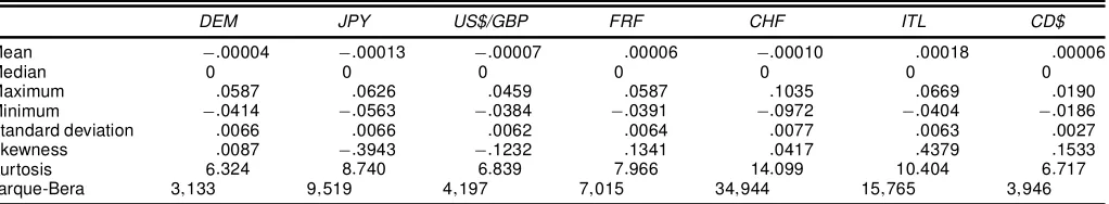
Before the test results for moving windows are reported, Ta-ble 3 presents descriptive statistics to highlight some charac-teristics of daily exchange rates throughout the January 1974– February 2001 period. Based on the average daily log exchange rate changes, it can be concluded that on average, US$ has depreciated against DEM, JPY, and CHF and has appreciated against GBP, FRF, CD$, and ITL. Daily exchange rate changes are not skewed one way or the other. All exchange rates have leptokurtic distribution. This is the reason behind the rejection of normality of daily log exchange rate changes by the Jarque– Berra test reported in the Table 3.
Table 4 presents the VRs along with the RS test and the heteroscedasticity-consistent multiple comparison test for the full sample using 2-, 4-, 8-, and 16-day return horizons. As the return horizon further increases, the number of nonoverlap-ping observations (1,000/return horizon) will decrease. Lo and MacKinlay (1989) showed that this will lead to a decline in the power of the VR test. For this reason, return horizons longer than 16 days are not considered. However, checked whether our results are sensitive to the choice of return horizon was checked, and it was determined that the results do not change signicantly when longer return horizons were included in the calculation of test statistics.
The VRs for all currencies are greater than 1, indicating the possibility of positive serial correlation in daily innovations to exchange rates. The MCT rejects the martingale property for the exchange rate of US$ against DEM, JPY, GBP, FRF, and CD$ at the 10% signicance level. The RS Wald test rejects the martingale hypothesis for these exchange rates at either the 5% or the 1% signicance level. It rejects the null hypothesis for the ITL exchange rate as well. Rejection of the martingale property for these currencies is not due to long return-horizons; the longest return-horizon considered is 16 days—much shorter than the size of the subsample windows.
Table 3. Descriptive Statistics for Daily Log Exchange Rate Changes (January 1974–February 2001)
DEM JPY US$/GBP FRF CHF ITL CD$
Mean ¡:00004 ¡:00013 ¡:00007 :00006 ¡:00010 :00018 :00006
Table 4. VR Test for Daily Log Exchange Rate Changes (January 1974–February 2001)
VR VR test statistic (z¤)
RS test
2 days 4 8 16 2 days 4 8 16 p value
DEM 1:03 1:044 1:078 1:149 1.983 1:563 1:758 2.30¤ :0159¤¤
JPY 1:036 1:061 1:091 1:2 1.936 1:85 1:838 2.85¤¤ <:0001¤¤
GBP 1:061 1:087 1:118 1:147 3.817¤¤ 2:927 2:521 2.136 <:0001¤¤
FRF 1:03 1:051 1:091 1:149 1.973 1:819 2:048 2.29¤ :0324¤¤
CHF 1:008 1:004 1:007 1:048 0.269 :079 :12 .595 :5214 ITL 1:042 1:063 1:081 1:151 2.207 1:76 1:49 1.997 :0012¤¤
CD$ 1:061 1:074 1:083 1:111 3.418¤¤ 2:336 1:715 1.601 <:0001¤¤ NOTE: Absolute maximum values of thez¤statistic (test statistics for the multiple comparison tests) are highlighted with bold characters.¤and¤¤ indicate the rejection of the null hypothesis at the 10% and 5% percent signicance levels.
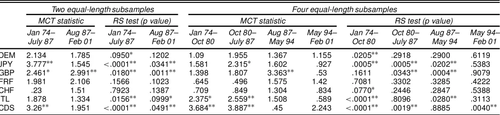
Approximately 27 years of daily data are used in the full-sample tests. So far, no study in the literature, has shown that these currencies (JPY, GBP, and CD$) have different character-istics than the others in the sample. On the contrary, as shown in Table 1, JPY/US$ and US$/GBP are the second and third lead-ing liquid exchange rates after DEM/US$. To check whether different results are obtained in different subperiods, martin-gale was tested for in two and four equal-length subperiods; the results are presented in Table 5.
As is the case with the full sample tests, the Wald test tends to reject martingale behavior in subsamples more often and more signicantly than the multiple comparison test. The results of both tests indicate that exchange rate behavior is not uniform throughoutthe oat. When the second half of the sample period is compared with the rst half, at least the RS test continues to reject martingale behavior for three exchange rates (DEM, JPY, and CD$) at the 5% signicance. Yet the intensity of the rejection of the martingale hypothesis tends to decline in the last two quarters of the oat period compared with the rst two quarters. The results also indicate that with the exception of the CD$, all exchange rates tend to follow martingale behavior since May 1994.
Together, the test results given in Tables 4 and 5 reveal that exchange rates might deviate from the martingale in some peri-ods but not in others. To obtain more evidence on the time se-ries behavior of exchange rate, both tests were applied to xed-length moving windows over the January 1974–February 2001 period. The xed length of the subsample windows was chosen as 1,000 daily observations, because Fong et al. (1997) showed that power performances of both tests improved substantially as the number of observations increased to 1,000.
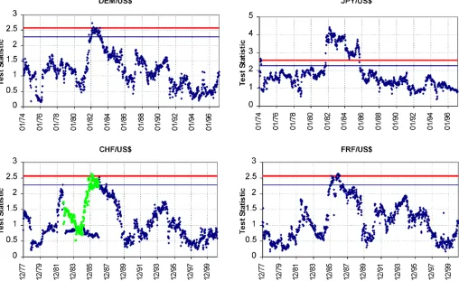
Figures 1–4 plot the joint VR test statistics on xed-length moving-subsample windows over the entire oat regime. The bold and normal straight lines in Figures 1 and 3 indicate the 5% and 10% signicance levels. The upper-level graphs in Figure 1 (for DEM and JPY exchange rates) are labeled with the starting date of the subsample windows, whereas the lower-level graphs (for CHF and FRF exchange rates) are labeled with the ending date of the moving-subsample windows. To give an example, the rst subsample starts in January 1974 and ends in December 1977.
The MCT statistics for bilateral exchange rates of US$ against DEM, JPY, CHF, and FRF presented in Figure 1 have some properties in common. MCT fails to reject the martingale hypothesis for these four exchange rates as long as the data for the 1970s are used. However, the MCT statistic for JPY is closer to the 10% rejection region over this period. As the subsam-ple window is moved to include the rst half of the 1980s, the MCT statistic for CHF and FRF increases close to the 10% crit-ical level as the subsample window is moved to include the data for 1982. Especially after June 1982, the Reagan administration had to intervene in the FX market to slow down the appreciation of the dollar. However, because the interventionsby the Federal Reserve did not take the form of coordinated intervention, the effect on the FX market was rather limited.
As the subsample windows are moved forward to include the data for the last quarter of 1985 in the subsample windows, test statistics show a signicant upward climb, reaching the rejec-tion region very quickly. This movement in the test statistics re-ects the effect of the Plaza Accord and the ensuing coordinated interventions by the major central banks in the FX markets. In-cluding this period in the subsample window leads to DEM and FRF increases to slightly above the critical level. The behavior
Table 5. VR-Based Tests on Daily Log Exchange Rate Changes (two and four equal-length subperiods of January 1974–February 2001)
Two equal-length subsamples Four equal-length subsamples
MCT statistic RS test (p value) MCT statistic RS test (p value)
Jan 74– Aug 87– Jan 74– Aug 87– Jan 74– Oct 80– Aug 87– May 94– Jan 74– Oct 80– Aug 87– May 94–
July 87 Feb 01 July 87 Feb 01 Oct 80 July 87 May 94 Feb 01 Oct 80 July 87 May 94 Feb 01
DEM 2:134 1:785 :0950¤ :1202 1:09 1:955 1:367 1:155 :0205¤¤ :2918 :2900 :6119
JPY 3:777¤¤ 1:545 <:0001¤¤ :0341¤¤ 1:581 2:315¤ 1:602 :927 :0005¤¤ :0005¤¤ :0202¤¤ :5383
GBP 2:461¤ 2:991¤¤ :0180¤¤ :0011¤¤ 1:398 1:807 3:363¤¤ :53 :1611 :0343¤¤ :0004¤¤ :9079
FRF 1:981 2:106 :1566 :1023 :645 :496 1:575 1:42 :7081 :3302 :3285 :4222 CHF :23 1:51 :7923 :1387 :709 :849 1:304 :834 :0770¤ :2446 :2847 :5388
ITL 1:878 1:334 :0156¤¤ :0999¤ 2:375¤ 2:559¤¤ 1:508 :589 <:0001¤¤ :8096 :0280¤¤ :3113
CDS 3:26¤¤ 1:951 <:0001¤¤ :0491¤¤ 3:684¤¤ 3:887¤¤ :45 2:243 <:0001¤¤ :0019¤¤ :8885 :0040¤¤ NOTE: ¤and¤¤indicate the rejection of the null hypothesis at the 10% and 5% signicance levels.
Figure 1. MCT on Fixed-Length Moving Windows With 1,000 Observations (January 1974–February 2001). Each dot corresponds to the MCT statistic for a particular subsample window. The bold and the normal straight lines indicate the 5% and 10% signicance levels. The upper graphs are labeled with the starting date of the subsample window, whereas the lower graphs are labeled with the ending date. The gray dots in CHF/US$ graph corresponds to the MCT statistics after the outliers of December 30–31, 1982 are dropped out.
of the MCT statistics for four major exchange rates leaves no doubt that the martingale property is rejected during the Plaza Accord period for these two currencies.
As the subsample windows continue to move forward, the MCT statistics for DEM and FRF start to decline and fall below the 10% critical region. Actually, for both currencies, the test statistics fall from 1.5 and above to 1.0 and below as the obser-vations for the Plaza Accord period are left out of the sample. In the case of DEM and FRF, the test statistics continue to stay below the rejection region for all other subsample windows con-sidered. However, when we move the subsample to include the observations during the Gulf War period and especially during and after the Desert Storm (February–March 1991), the MCT statistics for both exchange rates climb upward again.
Test results for JPY follow a similar pattern. MCT statis-tics for JPY reject the random walk more signicantly, and stay in the rejection region over a larger set of subsample win-dows. The test statistic stays above the 5% critical value un-til the observations pertaining to the Plaza Accord period are dropped out of the subsample window. The upward and down-ward jumps in the test statistic for JPY are very visible. How-ever, similar to DEM and FRF, JPY tends to move downward, well below the critical region, but only after the data pertaining to the Plaza Accord period are dropped out of the subsample windows. Based on Figure 1, it can be concluded that the im-pact of the coordinated interventions during the Plaza Accord
period lasted longer for the JPY exchange rate compared with other currencies.
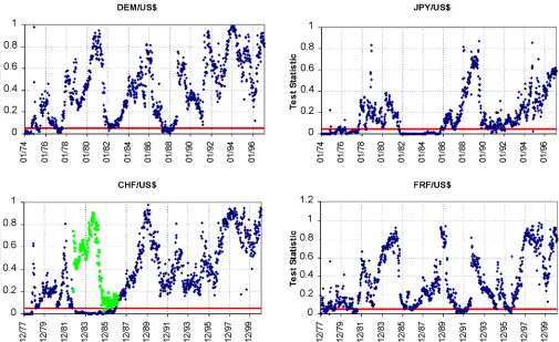
Figure 2 plots the marginal signicance level of the RS Wald test statistic for DEM, JPY, CHF, and FRF exchange rates. Comparing results for the two test statistics reveals that the RS Wald test rejects the martingale hypothesis more often and statistically more signicantly than MCT. For example, unlike MCT, the RS Wald test rejects the martingale hypothesis in the 1970s for all four exchange rates. This result is quite plausible given the power calculations reported by Fong et al. (1997) for the MCT and RS Wald tests. According to Fong et al. (1997), the RS Wald test has a higher power than the multiple com-parison test for AR(1) and fractionally integrated alternative hypotheses. Given the fact that the major central banks under-took frequent coordinated interventions throughout the 1970s (Schwartz 2000), the rejection of the martingale property by the RS Wald test throughout the 1970s is not surprising.
Besides these important differences in terms of the statistical signicance levels, plots of the two test statistics in Figures 1 and 2 lead to quite similar conclusions. In the rst place, for all four exchange rates, the RS Wald test moves into the rejection region as soon as the observations for the last quarter of 1985 are included in the moving-subsample windows. In the case of GBP, the test statistic stays in the rejection region for the rest of the subsample windows considered, perhaps except for those subsample windows ending in 1998.
Figure 2. RS Wald Test on Fixed-Length Moving Windows With 1,000 Observations (January 1974–February 2001). Each dot corresponds to the p value for the RS Wald test for a particular subsample window. The bold straight line indicates the 5% cutoff for the p value. The upper graphs are labeled with the starting date of the subsample window, whereas the lower graphs are labeled with the ending date. The gray dots in CHF/US$ graph corresponds to the p values of the RS test after the outliers of December 30–31, 1982 are dropped out.
Plottedpvalues for DEM and FRF are very similar, as was the case with their MCT statistics. In addition to the post-Plaza Accord period, the RS Wald test starts rejecting the martingale hypothesisonce the data for the Gulf War period are included in the dataset. In February and March 1991 (during and immedi-ately after the Operation Desert Storm) central banks intervened in the FX market. This episode is one of the examples where the MCT fails to reject the martingale property, whereas the RS Wald test rejects it at the 5% level. Even though the MCT sta-tistics for the two currencies also jump up with the inclusion of the data for the rst quarter of 1991, they do not reach the rejection region.
The MCT and RS test results for the CHF/US$ exchange rate show how sensitive both test procedures are to an outlier in the data. On the last two business days of December 1982, the CHF exchange rate realized the largest daily increase, followed by the largest daily decrease in its history. The CHF was 1.995 on December 29; it jumped by 10.9% to 2.2125 the next day, only to come down by 9.3% to 2.0075 on December 31st. This is not a mistake generated by our data, other sources of historical exchange rate series were checked for verication. Obviously, the rst difference of the log-CHF exchange rates for Decem-ber 30 and 31 displays a very strong negative correlation. When these two observations are included in the moving-subsample windows, the MCT falls from 1.46 to 0.76 and stays there as long as these two observations are included in the moving sub-sample. The RS test, in contrast, starts rejecting the martingale
hypothesis when these two observationsare included in the sub-sample. Thep value for the RS test drops from .48 to .024 as they are included in the subsample window, and it stay in the rejection region as long as the two observations are included in the subsample.
A search of the news accounts for the period revealed no ac-count of the particular cause of the CHF on December 30 and 31, 1982. To check how the test statistics for CHF would have behaved if the two outliers had not been in the sample, these outliers were dropped and the tests reapplied to the new sam-ple. The resulting MCT statistic and thepvalue for the RS Wald test are also presented in Figures 1 and 2 as the gray dots in the CHF panel. It is quite obvious from both graphs that once the two outliers are dropped out, the movement of the test statistics over time becomes quite similar to that of DEM and FRF before and after the Plaza Accord episode.
According to Figures 1 and 2, the test statistics tends to re-ject martingale hypothesis for all subsample windows of JPY during the coordinated intervention period that started after the Plaza Accord. JPY was also affected from the FX market inter-ventions during the Gulf War. However, unlike DEM, CHF, and FRF, JPY had a long period of diversion from the martingale property with the inclusion of the data for the post-1993 period in the subsample windows. The RS Wald test starts to reject the martingale hypothesis with thep value staying near or below the 20% level. This is the period when the Japanese economy went into the longest recession in its history.
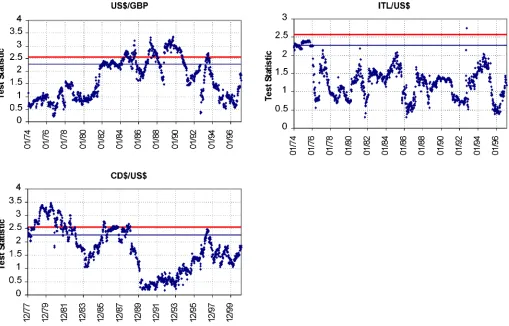
Figure 3. MCT on Fixed-Length Moving Windows With 1,000 Observations (January 1974–February 2001). Each dot corresponds to the MCT statistic for a particular subsample window. The bold and the normal straight lines indicate the 5% and 10% signicance levels. The upper graphs are labeled with the starting date of the subsample window, whereas the lower graphs are labeled with the ending date.
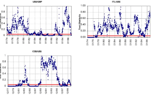
Next we move to Figures 3 and 4, where the MCT and RS test statistics for GBP, ITL, and CD$ are plotted. Test statistics for these three currencies follow different patterns compared with the four currencies discussed earlier. To start with, both the MCT and the RS Wald test cannot reject martingale behav-ior for GBP for the windows covering the 1970s. In addition, the test statistics for GBP after the mid-1980s differ from the exchange rates covered in Figures 1 and 2. Even though the test statistic turns downward as the last quarter of 1985 is dropped from the subsample window, this does not last long, and then it climbs up again and stays in the rejection region or very close to it with some ups and downs until very recently. It is cru-cial to observe that the MCT statistic for GBP climbs up to the rejection region during the Gulf War crisis and the ensuing cen-tral bank interventions in the FX markets in the second half of 1992. With the outbreak of the ERM crisis in September 1992, there is another upward jump in the test statistic to reject the martingale hypothesis. As the data pertaining to both October 1991 and September 1992 are dropped out of the sample, the test statistic moves away from the rejection region.
Both the MCT and RS Wald tests reject the martingale hy-pothesis for CD$ in the 1970s. The test statistics started to move away from the rejection region for the subsample windows cov-ering the early 1980s. However, with the coordinated interven-tions of the Plaza Accord period, both the MCT and RS Wald tests started to move to the rejection region indicating a strong
deviation from martingale behavior. Even though it was not af-fected by the Louvre Accord and the FX market intervention after the Gulf War, CD$ started to move away from martingale behavior as the data for the late 1996 and afterward are included in the subsample windows. In the late 1990s, the Canadian cen-tral bank followed a low interest rate policy, which led to a rapid decline in the value of the CD$.
The ITL exchange rate differs from others in certain aspects. The null hypothesis is rejected for the subsample windows cov-ering the 1970s. It was not signicantly affected during the Plaza Accord period. Both tests fail to reject the martingale hy-pothesis for the ITL over this period. The RS test rejects the martingale behavior when the data for the Gulf War period of early 1991 are included in the subsample window. Thepvalue for the RS test falls to the rejection region for a few subsample windows as soon as the data for the September 1992 ERM cri-sis are included. The RS test rejects the martingale hypothecri-sis for the ITL exchange rate when the data from late 1997 and all of 1998 are included in the subsample windows.
5. CONCLUSIONS
Previous research reached conclusions on the martingale property of exchange rates based on tests applied to a given sample or to its subsamples. This article has analyzed the daily behavior of major bilateral US$ exchange rates allowing for
Figure 4. RS Wald Test on Fixed-Length Moving Windows With 1,000 Observations (January 1974–February 2001). Each dot corresponds to the p value for the RS Wald for a particular subsample window. The bold straight line indicates the 5% cutoff for the p value. The upper graphs are labeled with the starting date of the subsample window, whereas the lower graphs are labeled with the ending date.
continuous change in the sample period. The empirical analy-sis used MCT and RS Wald test statistics to test for martingale hypothesis.
The analysis leads to several conclusions. First, the daily ex-change rate behavior is not uniform throughout the entire oat period. The bilateral US$ exchange rates against other major currencies do not follow the martingale behavior for the full duration of the oat regime. More specically, exchange rates tend to deviate from martingale behavior during the coordinated FX market interventions by central banks. In addition to in-terventionist period of the 1970s identify four such episodes: June–August 1982, when the Reagan administration changed its stance with respect to FX market interventions;the Plaza Ac-cord of September 1985; the Louvre AcAc-cord of February 1987; and immediately after the full-scale Gulf War in February– March 1991. The inclusion of the data for these episodes in the xed-length moving-subsample windows leads the test sta-tistics toward the rejection region.
Finally, responses of exchange rates to similar types of policy shocks (coordinated FX market intervention or the decision to leave the EMS) are not necessarily of the same intensity. For example, in terms of the effects of the FX market intervention on the behavior of exchange rates after the Plaza Accord, the exchange rates can be placed into two groups. Whereas DEM, FRF, and CHF diverged from martingale behavior temporarily after the Plaza Accord, the divergence of JPY, GBP, and CD$ from the martingale behavior was stronger and lasted longer.
In similar fashion, whereas the October 1992 departure from the EMS led to the divergence of the GBP from the martingale property for a long time, for the ITL there was only a slight temporary divergence from martingale behavior.
This study searched for indirect evidence that the time se-ries properties of daily exchange rates are inuenced by cen-tral bank interventions. Because the link between the cencen-tral bank interventions and the martingale behavior was not tested directly, the inuence of factors other than central bank inter-ventions cannot be ruled out. For that reason, the results herein should not be interpreted as implicating the central bank in-terventions to be the only cause of violation of the martingale property of daily exchange rates.
ACKNOWLEDGMENTS
The author thanks the editor, an associate editor, and two referees for very constructive comments and suggestions that helped improve the article signicantly. The author also thanks Emre Alper and seminar participants at Bogazici University for helpful comments.
[Received June 2001. Revised August 2002.]
REFERENCES
Anthony, M., and MacDonald, R. (1998), “On the Mean-Reverting Properties of Target Zone Exchange Rates: Some Evidence From the ERM,”European Economic Review, 42, 1493–1523.
Baillie, R. T., and Bollerslev, T. (1989), “Common Trends in a System of Ex-change Rates,”Journal of Finance, 44, 167–181.
Baillie, R. T., and Osterberg, W. P. (1997), “Central Bank Intervention and Risk in the Forward Market,”Journal of International Economics, 43, 483– 497.
Bank for International Settlements (1992),Triennial Central Bank Survey of Foreign Exchange and Derivatives Market Activity, Basel, Switzerland.
(1995),Triennial Central Bank Survey of Foreign Exchange and Derivatives Market Activity, Basel, Switzerland.
(1998),Triennial Central Bank Survey of Foreign Exchange and Derivatives Market Activity, Basel, Switzerland.
Catte, P., Galli, G., and Rebecchini, S. (1994), “Concerted Interventions and the Dollar: An Analysis of Daily Data,” inThe International Monetary System: Essays in the Memory of Rinaldo Ossola, eds. P. Kenen, F. Papadia, and F. Saccomanni, Cambridge, U.K.: Cambridge University Press, pp. 201–239. Chinn, M. D., and Meese, R. A. (1995), “Banking on Currency Forecasts: How
Predictable Is Change in Money?”Journal of International Economics, 38, 161–178.
Chow, K. V., and Denning, K. C. (1993), “A Simple Multiple Variance Ratio Test,”Journal of Econometrics, 58, 385–401.
Cochrane, J. (1991), “Volatility Tests and Efcient Markets,”Journal of Mone-tary Economics, 27, 463–485.
Diebold, F. X., and Chen, C. (1996), “Testing Structural Stability With Endoge-nous Breakpoint: A Size Comparison of Analytic and Bootstrap Procedures,”
Journal of Econometrics, 70, 221–241.
Diebold, F. X., Gardeazabal, J., and Yõlmaz, K. (1994), “On Cointegration and Exchange Rate Dynamics,”Journal of Finance, 49, 727–735.
Dominquez, K. M. (1990), “Market Responses to Coordinated Central Bank Intervention,”Carnegie-Rochester Conference Series on Public Policy, 32, 121–163.
(1998), “Central Bank Intervention and Exchange Rate Volatility,”
Journal of International Money and Finance, 17, 161–190.
(2001), “The Market Microstructure of Central Bank Intervention,” Working Paper 7337, National Bureau of Economic Research.
Fama, E. F., and French, K. R. (1988), “Permanent and Temporary Components of Stock Prices,”Journal of Political Economy, 96, 246–273.
Fong, W. M., Koh, S. K., and Ouliaris, S. (1997), “Joint Variance-Ratio Tests of Martingale Hypothesis for Exchange Rates,”Journal of Business and Eco-nomic Statistics, 15, 51–59.
Hahn, G. R., and Hendrickson, R. W. (1971), “A Table of Percentage Points of the Distribution of Large Absolute Value ofkStudenttVariates and Its Applications,”Biometrika, 58, 323–332.
Hochberg, Y. (1974), “Some Generalizations of T-Method in Simultaneous In-ference,”Journal of Multivariate Analysis, 4, 224–234.
Jegadeesh, N. (1991), “Seasonality in Stock Price Mean Reversion: Evidence From the U.S. and the U.K.,”Journal of Finance, 66, 1427–1444.
Liu, C. Y., and He, J. (1991), “A Variance-Ratio Test of Random Walks in For-eign Exchange Rates,”Journal of Finance, 46, 773–785.
Lo, A. W., and MacKinlay, A. C. (1988), “Stock Market Prices Do Not Fol-low Random Walks: Evidence From a Simple Specication Test,”Review of Financial Studies, 1, 41–66.
(1989), “The Size and Power of the Variance Ratio Test in Finite Sam-ples: A Monte Carlo Investigation,”Journal of Econometrics, 40, 203–238. Lothian, J. R. (1996), “Multi-Country Evidence on the Behavior of Purchasing
Power Parity Under the Current Float,”Journal of International Money and Finance, 16, 19–35.
Lothian, J. R., and Taylor, M. P. (1996), “Real Exchange Rate Behavior: The Recent Float From the Perspective of the Past Two Centuries,”Journal of Political Economy, 104, 488–509.
Mark, N. C. (1995), “Exchange Rates and Fundamentals: Evidence on Long-Horizon Predictability,”American Economic Review, 85, 201–218. Mark, N. C., and Sul, D. (2001), “Nominal Exchange Rates and Monetary
Fun-damentals: Evidence From A Small Post–Bretton Woods Panel,”Journal of International Economics, 53, 29–52.
McCallum, B. T. (1994), “A Reconsideration of the Uncovered Interest Parity Relationship,”Journal of Monetary Economics, 33, 105–132.
McKinnon, R. I. (1993), “The Rules of the Game: International Money in His-torical Perspective,”Journal of Economic Literature, 31, 1–44.
(1996),The Rules of the Game, Cambridge, MA: MIT Press. Meese, R. A., and Rogoff, K. (1983), “Empirical Exchange Rate Models of the
Seventies: Do They Fit Out of Sample?”Journal of International Economics, 14, 3–24.
Meredith, G., and Chinn, M. D. (1998), “Long-Horizon Uncovered Interest Rate Parity,” Working Paper 6797, National Bureau of Economic Research. Obstfeld, M. (1990), “The Effectiveness of Foreign-Exchange Intervention:
Re-cent Experience, 1985–1988,” inInternational Policy Coordination and Ex-change Rate Fluctuations, eds. W. H. Branson, J. A. Frenkel, and M. Gold-stein, Chicago: University of Chicago Press, pp. 197–237.
Papell, D. H. (1997), “Searching for Stationarity: Purchasing Power Parity Un-der the Current Float,”Journal of International Economics, 43, 313–332. Poterba, J. M., and Summers, L. H. (1988), “Mean Reversion in Stock Prices:
Evidence and Implications,”Journal of Financial Economics, 22, 27–59. Richardson, M., and Smith, T. (1991), “Tests of Financial Models in the
Pres-ence of Overlapping Observations,”Review of Financial Studies, 4, 227–254. Schwartz, A. (2000), “The Rise and Fall of Foreign Exchange Market
Interven-tion,” Working Paper 7751, National Bureau of Economic Research. White, H. (1980), “A Heteroscedasticity-Consistent Covariance Matrix
Estima-tor and a Direct Test for Heteroscedasticity,”Econometrica, 48, 817–838.