Full Terms & Conditions of access and use can be found at
http://www.tandfonline.com/action/journalInformation?journalCode=ubes20
Download by: [Universitas Maritim Raja Ali Haji] Date: 12 January 2016, At: 23:35
Journal of Business & Economic Statistics
ISSN: 0735-0015 (Print) 1537-2707 (Online) Journal homepage: http://www.tandfonline.com/loi/ubes20
Stock Market Downswing and the Stability of
European Monetary Union Money Demand
Kai Carstensen
To cite this article: Kai Carstensen (2006) Stock Market Downswing and the Stability of
European Monetary Union Money Demand, Journal of Business & Economic Statistics, 24:4, 395-402, DOI: 10.1198/073500106000000369
To link to this article: http://dx.doi.org/10.1198/073500106000000369
Published online: 01 Jan 2012.
Submit your article to this journal
Article views: 114
View related articles
Stock Market Downswing and the Stability of
European Monetary Union Money Demand
Kai C
ARSTENSENKiel Institute for the World Economy, Duesternbrooker Weg 120, 24105 Kiel, Germany (kai.carstensen@ifw-kiel.de)
This article analyzes the question whether money demand in the euro area underwent a structural change in the end of 2001 when M3 money growth started to considerably overshoot the reference value set by the European Central Bank. It is found that conventional specifications of money demand have in fact become unstable, whereas specifications that are augmented with equity returns and volatility remain stable. Using such an augmented specification, it turns out that the high M3 growth rates have not led to excess liquidity and thus do not pose a measurable threat to price stability.
KEY WORDS: Cointegration; Excess liquidity; Inflationary pressure; Stability test.
1. INTRODUCTION
On May 8, 2003, the European Central Bank (ECB) an-nounced a revision of its monetary policy strategy (European Central Bank 2003b). Most observers interpreted the revision as a weakening of the monetary pillar (de Grauwe 2003; Belke, Kösters, Leschke, and Polleit 2003). It might have been mo-tivated in part by the fact that M3 reference growth rates had been continuing to exceed the reference value of 4.5% by more than 2.5 percentage points since the end of 2001. At the same time, the ECB lowered its key interest rate from 4.25% on Au-gust 31, 2001 to 2% on June 6, 2003, even though the monetary developments suggested a raise in the interest rate.
The ECB attributed the strong money growth to portfolio shifts from equities to safe and liquid assets induced by the re-cent stock market downswing and the increased financial un-certainty and predicted that it would be reversed once stock prices rose again and uncertainty diminished (see, e.g., Euro-pean Central Bank 2003a). From this perspective, the recent money growth does not seem to pose a particular threat to price stability. It might, however, indicate that the relationship be-tween money and prices has become unstable and hence that money growth is not a well-suited tool for analyzing prospec-tive inflation and support monetary policy decisions. Then it would have been natural for the ECB to have reduced the weight of the monetary pillar.
Because it is generally assumed that money and prices are related through a money demand function, the preceding dis-cussion raises the question of whether European money demand has recently become unstable. Numerous papers have dealt with estimating money demand functions of the European Monetary Union (EMU) and testing their stability. Most used exclusively synthetic data for the pre-EMU period (e.g., Gottschalk 1999; Hayo 1999; Bruggeman 2000; Clausen and Kim 2000; Coenen and Vega 2001; Funke 2001; Müller and Hahn 2001; Golinelli and Pastorello 2002) or the period up to the first year of the EMU (Brand and Cassola 2000; Calza, Gerdesmeier, and Levy 2001) and cannot reject stability. Extending the dataset until the third quarter of 2001, Kontolemis (2002) found evidence for in-stability of the conventional money demand function at his very last observation due to the strong growth of M3 beginning in this period.
In a comprehensive stability analysis, Bruggeman, Donati, and Warne (2003) applied the fluctuation and Nyblom-type
stability tests proposed by Hansen and Johansen (1999) and ob-tained mixed results, but finally concluded that some specifi-cations of money demand seem stable. However, because their dataset ends with the fourth quarter of 2001 and the excessive money growth did not start until the second quarter of 2001, it is possible that their limited dataset prevented the statistical tests from indicating nonstability.
This article adds to the literature by first using an updated dataset for the period from the first quarter of 1980 to the second quarter of 2003, which provides more observations with exces-sive money growth at the end of the sample, and second, supple-menting the battery of existing stability tests with a new family of stability tests proposed by Andrews and Kim (2003) that fits the purpose of this article perfectly because it is designed to de-tect breakdown of cointegration at the end of a sample. Because it is found that a conventional money demand specification be-came unstable in 2001, an alternative money demand function is considered that is augmented by stock market variables. This money demand function exhibits structural stability and can be used to assess the importance of stock market developments on M3 growth rates. We provide evidence that the recent high M3 growth rates did not reflect excess liquidity that would have posed a threat to price stability.
The remainder of the article is organized as follows. Sec-tion 2 discusses the specificaSec-tion of the EMU long-run money demand function. Section 3 outlines various stability tests for cointegrated time series, and Section 4 presents the empirical estimation and testing results. Finally, Section 5 concludes.
2. SPECIFICATION OF LONG–RUN MONEY DEMAND
There already exists a large body of literature on specify-ing and estimatspecify-ing long-run European money demand functions and testing their stability. Detailed surveys have been provided by Fagan and Henry (1998) and Golinelli and Pastorello (2002). Concerning the specification issue, real money demand is gen-erally modeled as depending on real GDP as a scale variable,
© 2006 American Statistical Association Journal of Business & Economic Statistics October 2006, Vol. 24, No. 4 DOI 10.1198/073500106000000369
395
396 Journal of Business & Economic Statistics, October 2006
whereas there seems to be no consensus as to which opportunity cost measure should be included. Typical choices are a long-term (government bond) rate (Golinelli and Pastorello 2002), a short-term (money market) rate (Brand and Cassola 2000; Funke 2001; Kontolemis 2002), or a spread between long-term and short-term rates, with the latter used to approximate the own rate of M3, that is, the rate of return on M3 (Gottschalk 1999; Clausen and Kim 2000; Müller and Hahn 2001). Calza et al. (2001) argued that it would be better to construct a di-rect measure of the own rate and use the spread between a short-term rate and this own rate, an approach also followed by Bruggeman et al. (2003). A few authors have included ad-ditional variables, such as the inflation rate (Coenen and Vega 2001) or real stock prices (Kontolemis 2002; Bruggeman et al. 2003).
In this article we follow Calza et al. (2001) and consider the baseline long-run money demand function
mpt=β1yt+β2(rst−rto)+ut, (1) wherempt=mt−ptdenotes real M3,yt is real GDP,rtois the own rate of M3,rst is the short-term interest rate, andut is the disequilibrium. This choice of an opportunity cost variable is motivated by two factors. First, it has been successfully ap-plied in the most recent work (Calza et al. 2001; Bruggeman et al. 2003); second, Calza et al. (2001) obtained an insignifi-cant effect of the spread between a long rate and the own rate on money demand. A comprehensive analysis of different pos-sible specifications reported in an earlier version of this article (available from the author on request) found that the spread be-tween the short rate and the own rate is an appropriate choice in terms of significance and economic interpretation.
Concerning the stability of European money demand, most authors apply informal techniques, such as recursive estimation and out-of-sample forecasting or Chow tests with critical values valid only for stationary relationships. In contrast, Funke (2001) used the SupF test of Hansen (1992) designed for cointegrating regressions, and Bruggeman et al. (2003) used the fluctuation and Nyblom tests of Hansen and Johansen (1999) developed for cointegrated vector autoregression (VAR) models. Rather surprisingly, there seems to be consensus that European money demand functions are remarkably stable (see, e.g., Calza and Sousa 2003 for a discussion of this result). However, the sam-ples analyzed so far generally end before the recent start of ex-cessive money growth rates. Two notable exceptions are those reported by Kontolemis (2002), who found signs of instability at his last observation 2001Q3, and Bruggeman et al. (2003), who could not reject stability in a sample ending in 2001Q4 but obtained a strong rise in the money overhang in 2001Q4.
In fact, the persistently high money growth rates since 2001 might indicate instability of a money demand function that ne-glects stock market influences. This view is supported by an empirical analysis of the ECB (2003a), which reveals that shifts of risky assets into funds that are part of M3 compose a large fraction of money growth. The coincidence of excessive money growth and stock market turmoil suggests that there might be a relationship between money demand and stock prices.
Friedman (1988) argued that stock markets should affect money demand in several ways; for instance, real stock prices should have a positive wealth effect, stock returns should have
a negative substitution effect, and stock market risk should have a positive risk-avoidance effect given risk-averse agents. For the United States, Friedman can support these claims empiri-cally. Choudhry (1996) and Carpenter and Lange (2002) also found evidence in favor of a long-run influence of stock mar-ket variables on U.S. money demand. Caruso (2001) extended this work to a panel of 25 countries and obtained a significant wealth effect. For EMU money demand, Kontolemis (2002) found a significant long-run influence of stock prices, whereas Bruggeman et al. (2003) did not obtain significant of effects either real stock prices or stock market volatility. The latter re-sult stands in contrast to the argument of the ECB (2003a) that the increased uncertainty in equity markets has led to portfolio shifts from equities to safe and liquid assets, which are part of M3, and hence to the excessive M3 growth. Moreover, Cassola and Morana (2002) found that real stock prices play an impor-tant role in the monetary transmission mechanism.
To analyze the impact of stock market variables on money demand, the “stock market” specification
mpt=β1yt+β2(rst−rto)+β3(rte−rot)+β4vt+ut (2) is used, whereret denotes equity returns and vt denotes stock market volatility. (Again, a more comprehensive analysis of dif-ferent stock market specifications is available on request.) The-oretically, the stock market variables should reflect expectations of investors who decide whether they want to hold money or equity. However, there does not seem to be a well-suited expec-tation variable for the period since 1980. Using realized future returns instead would not only impose rational expectations on stock market investors, but also would necessitate generalized method-of-moments GMM estimation, which is not readily available for a cointegrated VAR model. Therefore, backward-looking variables are included, with the obvious problem that past outcomes might not be an optimal predictor of the future outcomes with which investors are concerned. There are, how-ever, two observations that may justify this choice in addition to the simple availability rationale. First, if stock market variables behave like a random walk, then current values are as good as any predictor. Second, historical performance measures play a significant role in stock market practice. In particular, it seems that the recent stock market downturn has had a protracted im-pact on money demand, which may be explained by investors revising their expectations only gradually over time as more in-formation is observed. Moreover, from an econometric perspec-tive, the long-run analysis should be invariant to using realized current versus expected future variables as long as the differ-ence between them is stationary.
3. TESTS FOR LONG–RUN
STRUCTURAL STABILITY
It has long been recognized that the variables entering the long-run money demand functions (1) or (2) can be modeled as integratedI(1)processes. Therefore, stability of a money de-mand function requires at a minimum that it constitute a coin-tegration relationship. It is by now a well-established empirical finding that the European money demand function is stable and cointegrated at least for the sample 1980Q1–1998Q4, which we will call the baseline sample here. Therefore, it is particularly
interesting to test whether this stability has been lost since then, especially in the time since M3 started its excessive growth. To-ward this end, tests for long-run stability are applied, as briefly reviewed in what follows.
Long-run stability means that the parameters of the coin-tegration relationship are invariant over time. To allow valid inference, the stability tests must take into account the nonsta-tionarity of the single variables. For cointegrated VAR models, Hansen and Johansen (1999) suggested applying a fluctuation test to the nonzero eigenvalues of the reduced-rank matrix and a Nyblom test to the cointegration parameters. The fluctuation test is in the spirit of Ploberger, Krämer, and Kontrus (1989) and rejects stability when the recursively estimated eigenvalues fluctuate excessively. It can be applied either to the eigenval-uesλi themselves, giving rise to the test statistic Supλ, or to the transformationξi=log(λi/(1−λi)), giving rise to the test statistic Supξ. The Nyblom test statistics MeanQ and SupQ are obtained by applying the mean and supremum operators, respectively, to the recursively estimated likelihood maximum (LM) statistics for structural stability of the cointegration pa-rameters. Hansen and Johansen (1999) used a first-order ap-proximation to the relevant score function to calculate the LM statistic, whereas Bruggeman et al. (2003) used the score func-tion itself, which yields the test statistics MeanQs and SupQs. Bruggeman et al. (2003) and Warne (2005) suggested that the MeanQsand SupQstests are superior to the MeanQ and SupQ tests because the latter suffer from numerical problems in sim-ulation exercises, leading to small-sample distributions that are far away from the limit distributions. Therefore, the results of the MeanQ and SupQ tests should be taken with caution.
Usually, it is deemed a particular strength of all of these tests that they do not require a prespecified break date, but rather test the null hypothesis of structural stability against the alter-native that there is a structural break at some unknown point in the sample. For the present situation, this strength may turn out to be of less value, because stability in the pre-EMU period is well documented (Calza and Sousa 2003), whereas there are two known dates later in the sample when instability may show up, namely the start of EMU in 1999Q1 and the start of ex-cessive M3 growth around 2001Q4. Although the former date is clearly identified exogenously, one can argue that the latter is not, and that it cannot be unambiguously fixed to exactly one quarter. On the other hand, there is ample evidence from newspapers, ECB reports, commentators, and other sources that something was happening on around this date. Therefore, tests that use the information that there was a break at the end of the sample, probably around 2001Q4, might be better suited than tests that abstract from any a priori knowledge.
Unlike the fluctuation and Nyblom tests, the cointegration breakdown tests proposed by Andrews and Kim (2003) are particularly well suited to the situation of a potential break at the end of the sample. The cointegration breakdown tests are generalizations of the well-known Chow stability test and can be applied to any estimation procedure, such as fully mod-ified ordinary least squares (FM–OLS) proposed by Phillips and Hansen (1990) and full information maximum likelihood (FIML) proposed by Johansen (1988, 1991). Moreover, critical values andpvalues can be obtained from parametric subsam-pling, which circumvents the use of asymptotic distributions.
This article applies thePc andRc statistics that Andrews and Kim (2003) found to have stable sizes and good power proper-ties for detecting the breakdown of a cointegration relationship at the end of a sample, due to either a shift in the parameter vector of the cointegration relationship or a change in the dis-tribution of the cointegration residuals from being stationary to being integrated,I(1).
4. EMPIRICAL ANALYSIS
This section presents and compares the empirical results for the baseline and the stock market specifications of the euro area money demand function. First, cointegration and long-run sta-bility tests are used to determine a stable long-run money de-mand relationship. Then the question is analyzed whether the recent strong money growth has created excess liquidity in the euro area. The sample runs from 1980Q1 to 2003Q2, with the first four observations reserved as presample values. The construction of the variables is explained in the Appendix.
4.1 Cointegration and Long-Run Stability
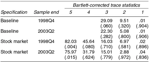
The cointegration properties of the baseline and stock market specifications in both the baseline and the full sample are ana-lyzed by Bartlett-corrected trace tests (Johansen 2002). Toward this end, VAR models with an unrestricted constant were esti-mated. (The results are robust to adding a linear trend restricted to the cointegration space.) For both models, a lag order of two was picked by the Schwarz and Hannan–Quinn information cri-teria, which was sufficient to obtain uncorrelated residuals, as indicated by LM tests for first- and fourth-order autocorrelation. Table 1 reports the trace test results along withpvalues derived from the asymptotic distribution. Using bootstrappedpvalues instead did not lead to any important changes, however. At the 10%, but not at the 5%, level, the variablesmpt,yt, andrst −rot of the baseline specification exhibited one cointegration rela-tionship in the baseline sample; however, the null of no coin-tegration could not be rejected in the full sample. This can be taken as a first sign of the long-run instability of this specifica-tion. In contrast, the variablesmpt,yt,rst −rot,ret −rto, andvt of the stock market specification were clearly cointegrating in both samples.
Imposing a cointegration rank of 1, the long-run parame-ters can be estimated by FIML. As a cross-check, FM–OLS
Table 1. Cointegration of the Long-Run Money Demand Specifications
Bartlett-corrected trace statistics Specification Sample end 5 4 3 2 1
Baseline 1998Q4 29.09 9.51 .01 (.060) (.320) (.904) Baseline 2003Q2 22.30 5.08 .01
(.282) (.800) (.906) Stock market 1998Q4 82.03 45.64 16.03 6.97 .02
(.004) (.080) (.710) (.581) (.896) Stock market 2003Q2 75.97 31.79 15.01 2.88 .04
(.015) (.624) (.779) (.972) (.836)
NOTE: The baseline and stock market specifications are given in (1) and (2). The
Bartlett-corrected trace statistics proposed by Johansen (2002) are obtained from a VAR model with two
lags, which is sufficient to guarantee uncorrelated disturbances. The asymptoticpvalues of the
trace tests are given in parentheses. The computations are performed using Anders Warne’s program Structural VAR 0.24.
398 Journal of Business & Economic Statistics, October 2006
Table 2. Estimation of the Long-Run Money Demand Specifications
Estimated parameters Specification Sample end Estimation method β1 β2 β3 β4
Baseline 1998Q4 FM–OLS 1.37 −.54 (.049) (.367) FIML 1.32 −.94 (.036) (.279) 2003Q2 FM–OLS 1.40 −.72 (.099) (.821) FIML 1.09 −3.40 (.083) (.697)
Stock market 1998Q4 FM–OLS 1.30 −1.40 −.09 0 (.043) (.412) (.047) (.011)
NOTE: The baseline and stock market specifications are given in (1) and (2). FM–OLS denotes fully modified least
squares. The nonparametric correction is calculated using a Parzen kernel with associated automatic bandwidth se-lection as proposed by Hansen (1992). FIML denotes the full information maximum likelihood estimator (Johansen 1988, 1991) with lag length 2 to obtain uncorrelated residuals and cointegration rank 1. Standard errors are reported in parentheses.
estimates are reported in Table 2 as well. First, consider the baseline specification. The FIML estimates changed from 1.32 (baseline sample) to 1.09 (full sample) forβ1and from−.94
(baseline sample) to −3.40 (full sample) for β2. Again, this
finding informally indicates long-run instability. Although the FM–OLS point estimates remained rather stable, the estimated standard errors increased considerably, again pointing to poten-tial stability problems. The estimated parameters of the stock market specification changed much less than the parameters of the baseline specification, especially when taking estima-tion uncertainty into account. Except for the FM–OLS estimate of β4 in the baseline sample, all parameters were highly
sig-nificant and correctly signed. The income elasticity of slightly below 1.30 is in the range obtained in previous studies, whereas the interest rate semielasticity is rather large in absolute terms. Moreover, in line with findings of Friedman (1988), long-run money demand is negatively related to equity returns and posi-tively related to stock market volatility.
After imposing a cointegration rank of 1, the stability of the two specifications was analyzed by the eigenvalue fluctu-ation and Nyblom tests. Thep values of these tests were de-rived from a parametric bootstrap, which provides stable sizes in small samples, as documented by Warne (2005) in an ex-tensive Monte Carlo study. Toward this end, the VAR was es-timated using the cointegration rank of 1, which yielded the estimated mean parametersBˆ and the estimated covariance
ma-trixˆ. In each bootstrap replication, normally distributed dis-turbances with mean0and covariance matrix ˆ were drawn.
(A bootstrap procedure that resamples directly from the residu-als led to virtually the same results.) Then the bootstrap distur-bances, the actual initial values, and the parametersBˆwere used
to generate a bootstrap sample,Yb
t,t=1980Q1, . . . ,2003Q2, from which a bootstrap test statistic was calculated. Bootstrapp values for each actual test statistic were based on 999 bootstrap replications, as suggested by MacKinnon (2002).
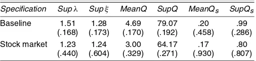
The results of the stability tests are displayed in Table 3. For both the baseline specification and the stock market specifica-tion, stability cannot be rejected using any test. Note that the
MeanQ and SupQ statistics are very large, indicating that the numerical problems found by Warne (2005) also show up here. Nevertheless, because the remaining four tests do not reject stability either, the test results suggest that either both speci-fications are stable or the null hypothesis of stability cannot be rejected because of low power, as would be typical of situations in which the break occurs at the end of the sample.
More evidence can be gained from the cointegration break-down tests of Andrews and Kim (2003), which were applied to FIML and FM–OLS estimation of the cointegration parame-ters. Three different test setups were evaluated. First, a break after the start of EMU 1999Q1 was tested in a reduced sam-ple that ends at 2001Q3, that is, before the M3 growth rates become extremely large. Thus a potential break after 2001Q3 did not affect the test. The results reported in Table 4 clearly show that the start of EMU did not induce a break for any of the two specifications. Next, the break after the start of EMU was tested in the full sample ending at 2003Q2 and thus includ-ing the excessive M3 growth rates. In this case, stability of the baseline specification was rejected by the tests applied to FM– OLS at the 10% level and FIML at the 1% level, indicating that
Table 3. Nyblom and Fluctuation Tests of the Long-Run Money Demand Specifications
Specification Supλ Supξ MeanQ SupQ MeanQs SupQs
Baseline 1.51 1.28 4.69 79.07 .20 .99 (.168) (.173) (.170) (.192) (.458) (.286) Stock market 1.23 1.24 3.00 64.17 .17 .80
(.440) (.604) (.329) (.271) (.930) (.807)
NOTE: The baseline and stock market specifications are given in (1) and (2). MeanQ and
SupQ denote the Nyblom tests based on a first-order Taylor expansion of the score function
as proposed by Hansen and Johansen (1999), MeanQsand SupQsdenote the related Nyblom
tests based directly on the score function as proposed by Bruggeman et al. (2003). Supλand
Supξdenote the fluctuation tests based on the largest eigenvalueλ1and the transformation
ξ1=log (λ1/(1−λ1)), as proposed by Hansen and Johansen (1999). All test statistics are com-puted from a VAR model with two lags and cointegration rank 1. The first 16 observations are
used as the base period, as done by Hansen and Johansen (1999, p. 316). Bootstrappedp
val-ues calculated with Anders Warne’s program Structural VAR 0.24 are given below the test sta-tistics.
Table 4. Cointegration Breakdown Tests of the Long-Run Money Demand Specifications
Specification Sample end Break Pc(FM) Rc(FM) Pc(FIML) Rc(FIML)
Baseline 2001Q3 1999Q1 .968 .999 .952 .999 2003Q2 1999Q1 .055 .073 0 0 2003Q2 2001Q4 0 0 0 0 Stock market 2001Q3 1999Q1 .936 .999 .613 .323
2003Q2 1999Q1 .964 .655 .655 .200 2003Q2 2001Q4 .753 .662 .156 .052
NOTE: The baseline and stock market specifications are given in (1) and (2).PcandRcare the cointegration
break-down tests proposed by Andrews and Kim (2003). They are based either on estimation of a VAR with two lags and cointegration rank 1 (FIML) or on fully modified least squares with Parzen kernel and associated automatic bandwidth
selection (FM). Only the simulatedpvalues are reported, because the simulated critical values change from case to
case so that the test statistics themselves are difficult to interpret.
the break occurred at the end of the sample after 2001Q3. This can be confirmed be testing the break point of 2001Q4 in the full sample. All four tests reject stability of the baseline speci-fication at the 1% level. In contrast, at the 10% level, stability cannot be rejected for the stock market specification except for theRc(FIML) test, which has a p value of .052 and thus is a borderline case.
Hence, from the tests of long-run stability it can be concluded that there are strong signs of instability for the baseline specifi-cation that neglects any stock market influence on EMU money demand. On the other hand, the extended specification that in-cludes equity yields and stock market volatility is stable by all of the criteria applied.
4.2 Excess Liquidity
The strong rise in money growth in the euro area in recent years has provoked the concern that excess liquidity has built up, with the possible consequence that inflation will start to rise in the near future. This concern is based mainly on a particu-larly simple measure of excess liquidity, namely the difference between the actual money growth rates and the reference value of 4.5% announced by the ECB (1999). Because actual money growth rates have permanently exceeded 4.5% since the end of 2001, this approach indicates that there is enormous excess liquidity in the euro area. The reference value was derived by the ECB from the quantity equation using the desired inflation rate and assumed long-run growth rates in output and velocity that resemble the historical averages before the monetary union; however, there is no reason why historical averages should be good indicators for the current situation.
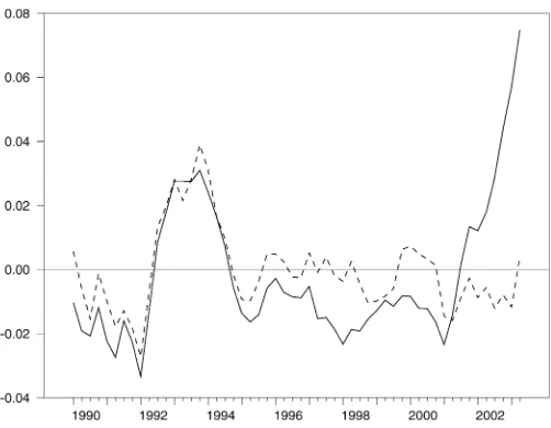
An alternative measure of long-run excess liquidity is the money overhang. Money overhang is defined as the difference between the observed money balance and the estimated equi-librium money demand and thus is derived from an equiequi-librium concept that takes the current situation into account (Masuch, Pill, and Willeke 2001; Nicoletti-Altimari 2001). Figure 1 com-pares two measures of money overhang, the first estimated from the baseline specification and the second estimated from the stock market specification. In both cases, the FM–OLS esti-mates were used because they are more stable in the base-line specification. It turns out that neglecting the stock market influence would indicate that there has been a strong money overhang since the end of 2001, peaking at nearly 8% in 2003Q2. This number compares well with the results of other authors who neglected stock market influences (e.g., Belke et al.
2004). However, the strong money overhang may simply reflect the cointegration breakdown of the baseline specification after 2001. In fact, money overhang is negligible if the money de-mand function includes the stock market variables. This finding is consistent with the view that the recent excessive M3 growth rates can be attributed to the stock market downswing. Once stock market developments are taken into account, there is no indication that there is excess liquidity and, thus, serious infla-tionary pressure in the euro area.
5. CONCLUSION
This article has analyzed the stability properties of two money demand specifications for the euro area. Using, in-ter alia, cointegration breakdown tests recently introduced by Andrews and Kim (2003), the hypothesis of structural stabil-ity had to be rejected when stock market influences were ne-glected in long-run money demand. The tests indicate that the break point was probably at the end of the year 2001, when M3 growth increased and stock market conditions deteriorated. However, including equity returns and stock market volatility in the long-run money demand equation improved stability con-siderably.
The presence of excess liquidity was analyzed by means of the money overhang, defined as the difference between the ob-served money balances and the estimated long-run money de-mand. It turns out that the conventional measure, which neglects
Figure 1. Money Overhang From 1990Q1 to 2003Q2 ( baseline specification; stock market specification).
400 Journal of Business & Economic Statistics, October 2006
the influence of the stock market variables, indicates an alarm-ingly high money overhang, whereas the more appropriate mea-sure incorporating the influence of the stock market variables does not indicate any noteworthy excess liquidity. This result corroborates the view put forward by the ECB that the recent money growth poses no exceptional threat to price stability.
Overall, the results demonstrate that measures of excess liq-uidity produce different results depending on whether stock market variables are included. Because the official 4.5% money growth target was derived without taking stock market influ-ences into account, it is no wonder that this target is misleading in the current environment. It was perhaps due to this realiza-tion that the ECB decided to downweight the monetary pillar in their May 2003 policy revision.
ACKNOWLEDGMENTS
The author thanks, without implicating, Don Andrews, Paul Kramer, Joachim Scheide, Anders Warne, Beatrice Weder, the editor, Torben Andersen, three unknown referees, and the par-ticipants of theFreitagsseminarat the Bundesbank for helpful comments and suggestions.
APPENDIX: CONSTRUCTION OF THE DATA
The dataset published by Calza et al. (2001), which con-tains data for M3, GDP, the GDP deflator, the long-term and short-term interest rates, and the own rate of M3 for 1980Q1 to 1999Q4, was updated until 2003Q2. To not induce a break in the data series, their construction of variables was closely mim-icked. M3 was updated with flows adjusted for any changes that did not arise from transactions. This implies in particular that the break induced by EMU enlargement in 2001 was eliminated from the data. In a similar manner, GDP and its price deflator
were updated by adding log changes to the last observation of the Calza et al. (2001) dataset. Again, the EMU enlargement break was eliminated by using log changes of EMU-11 before enlargement and of EMU-12 after enlargement. The short-term and long-term interest rates were updated with the 3-month money market rate and the 10-year government bond yield. Fi-nally, the own rate of M3 was constructed from the rates of re-turn to the components of M3 as outlined by Calza et al. (2001). The data for M3 and the interest rates from 2000Q1 to 2003Q2 were taken from the ECB website, and the data for GDP and the GDP deflator were taken from Eurostat, through Datastream.
Nominal stock prices were approximated using the German DAX30 for 1980–1986 (because no euro-denominated Euro-pean stock price index is available for this period) and the Dow Jones Euro Stoxx50 for 1987–2003. The data were downloaded from Datastream. The DAX30 was rescaled such that the value on December 31, 1986 equaled the value of the Euro Stoxx50 on January 1, 1987. Equity returns were constructed as fol-lows. First, the annualized log difference of average quarterly stock prices were calculated, which yielded a very volatile se-ries. Therefore, a 3-year average of the equity returns was com-puted. This rather long-term yield measure was used to mimic the fundamental yield path and exclude erratic short-term yield changes, which probably do not affect long-run money demand. Because there are clearly many ways to obtain a smooth quar-terly series of equity returns from daily data, the following al-ternatives were checked: a 3-year average of quarterly returns calculated as the quarterly average of daily returns, and a 2-year and a 2-12–year average instead of a 3-year average. In all cases, the estimation results remained largely unaffected.
Stock market volatility was constructed as the 2-year average of the conditional variance estimated from a leverage gener-alized autoregressive heteroscedasticity (GARCH) model with
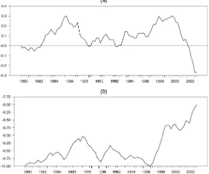
(a)
(b)
Figure 2. The Stock Market Variables From 1980Q1 to 2003Q2. (a) Equity returns. (b) Stock market volatility.
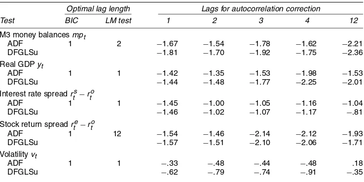
Table A.1. Univariate Unit Root Tests
Optimal lag length Lags for autocorrelation correction
Test BIC LM test 1 2 3 4 12
M3 money balancesmpt
ADF 1 2 −1.67 −1.54 −1.78 −1.62 −2.21
NOTE: ADF is the augmented Dickey–Fuller test, and DFGLSu is the Dickey–Fuller test with GLS detrending proposed by Elliott (1999).
The test regressions formptandytwere estimated with a constant and a linear trend. The corresponding 5% critical values are−3.45 for
ADF and−3.17 for DFGLSu. The test regressions forrtts−rto,rte−rto, andvtwere estimated with a constant. The corresponding 5% critical
values are−2.89 for ADF and−2.73 for DFGLSu. The optimal lag length of the ADF model was determined both by the Bayesian information
criterion (BIC) and by successively increasing the lag length until the null of no autocorrelation could not be rejected using an LM test (LM).
t-distributed innovations, applied to daily returns of the nomi-nal stock price index. Using averages makes the volatility index less erratic and better reveals the underlying movement in risk perception, which again seemed a better measure to include in a long-run money demand function. Further, the sensitivity of the results was also rechecked, with the degree of smoothing changed to 2-12–year and 3-year averages. The estimation re-sults remained unaffected. The two stock market variables are displayed in Figure 2.
The presence of unit roots is a necessary condition for a vari-able to enter a cointegration relationship. Because standard unit root tests fail to reject the unit root assumption for all variables in Table A.1, we treat these variables as integrated of order 1. The volatility measure in Table A.1 was constructed from a GARCH model with a nearly nonstationary conditional vari-ance equation, hence the result of the unit root tests is no sur-prise. (For a discussion of the nonstationarity of interest rate spreads, see Calza et al. 2001; Evans and Lewis 1994.)
[Received April 2005. Revised April 2006.]
REFERENCES
Andrews, D. W. K., and Kim, J.-Y. (2003), “End-of-Sample Cointegration Breakdown Tests,” Discussion Paper 1404, Cowles Foundation.
Belke, A., Kösters, W., Leschke, M., and Polleit, T. (2003), “Challenges to ECB Credibility,” Observer no. 5, European Central Bank.
(2004), “Liquidity on the Rise: Too Much Money Chasing Too Few Goods,” Observer no. 6, European Central Bank.
Brand, C., and Cassola, N. (2000), “A Money Demand System for Euro Area M3,” Working Paper 39, European Central Bank.
Bruggeman, A. (2000), “The Stability of EMU-Wide Money Demand Func-tions and the Monetary Policy Strategy of the European Central Bank,”
Manchester School, 68, 184–202.
Bruggeman, A., Donati, P., and Warne, A. (2003), “Is the Demand for Euro Area M3 Stable?” Working Paper 255, European Central Bank.
Calza, A., Gerdesmeier, D., and Levy, J. (2001), “Euro Area Money Demand: Measuring the Opportunity Costs Appropriately,” Working Paper 01/179, In-ternational Monetary Fund.
Calza, A., and Sousa, J. (2003), “Why Has Broad Money Demand Been More Stable in the Euro Area Than in Other Economies? A Literature Review,” in
Background Studies for the ECB’s Evaluation of Its Monetary Policy Strat-egy, ed. O. Issing, Frankfurt: European Central Bank, pp. 229–243.
Carpenter, S. B., and Lange, J. (2002), “Money Demand and Equity Markets,” Working Paper 2003-3, FEDS.
Caruso, M. (2001), “Stock Prices and Money Velocity: A Multi-Country Analy-sis,”Empirical Economics, 26, 651–672.
Cassola, N., and Morana, C. (2002), “Monetary Policy and the Stock Market in the Euro Area,” Working Paper 119, European Central Bank.
Choudhry, T. (1996), “Real Stock Prices and the Long-Run Money Demand Function: Evidence From Canada and the USA,”Journal of International Money and Finance, 15, 1–17.
Clausen, V., and Kim, J.-R. (2000), “The Long-Run Stability of European Money Demand,”Journal of Economic Integration, 15, 486–505.
Coenen, G., and Vega, J.-L. (2001), “The Demand for M3 in the Euro Area,”
Journal of Applied Econometrics, 16, 727–748.
de Grauwe, P. (2003), “The Central Bank That Has Missed the Point,”Financial Times, May 13.
European Central Bank (1999), “The Stability-Oriented Monetary Policy Strat-egy of the Eurosystem,”ECB Monthly Bulletin, January, 39–50.
(2003a), “Economic Developments in the Euro Area,”ECB Monthly Bulletin, May, 9–29.
(2003b), “The ECB’s Monetary Policy Strategy,” European Central Bank press release, May, 8.
Elliott, G. (1999), “Efficient Tests for a Unit Root When the Initial Observa-tion Is Drawn From Its UncondiObserva-tional DistribuObserva-tion,”International Economic Review, 40, 767–783.
Evans, M. D. D., and Lewis, K. K. (1994), “Do Stationary Risk Premia Explain It All? Evidence From the Term Structure,”Journal of Monetary Economics, 33, 285–318.
Fagan, G., and Henry, J. (1998), “Long-Run Money Demand in the EU: Evi-dence From Area-Wide Aggregates,”Empirical Economics, 23, 483–506. Friedman, M. (1988), “Money and the Stock Market,” Journal of Political
Economy, 96, 221–245.
Funke, M. (2001), “Money Demand in Euroland,”Journal of International Money and Finance, 20, 701–713.
Golinelli, R., and Pastorello, S. (2002), “Modelling the Demand for M3 in the Euro Area,”European Journal of Finance, 8, 371–401.
Gottschalk, J. (1999), “On the Monetary Transmission Mechanism in Europe,”
Journal of Economics and Statistics, 219, 357–374.
Hansen, B. E. (1992), “Tests for Parameter Instability in Regressions WithI(1) Processes,”Journal of Business & Economic Statistics, 10, 321–335. Hansen, H., and Johansen, S. (1999), “Some Tests for Parameter Constancy in
Cointegrated VAR Models,”Econometrics Journal, 2, 306–333.
Hayo, B. (1999), “Estimating a European Demand for Money,”Scottish Journal of Political Economy, 46, 221–244.
Johansen, S. (1988), “Statistical Analysis of Cointegration Vectors,”Journal of Economic Dynamics and Control, 12, 231–255.
(1991), “Estimation and Hypothesis Testing of Cointegrating Vectors in Gaussian Vector Autoregression Models,”Econometrica, 59, 1551–1580. (2002), “A Small-Sample Correction of the Test for Cointegration Rank in the Vector Autoregressive Model,”Econometrica, 70, 1929–1962.
402 Journal of Business & Economic Statistics, October 2006
Kontolemis, Z. G. (2002), “Money Demand in the Euro Area: Where Do We Stand (Today)?” Working Paper 02/185, International Monetary Fund. MacKinnon, J. G. (2002), “Bootstrap Inference in Econometrics,”Canadian
Journal of Economics, 35, 615–645.
Masuch, K., Pill, H., and Willeke, C. (2001), “Framework and Tools of Monetary Analysis,” inMonetary Analysis: Tools and Applications, eds. H.-J. Klöckers and C. Willeke, Frankfurt: European Central Bank. Müller, C., and Hahn, E. (2001), “Money Demand in Europe: Evidence From
the Past,”Kredit und Kapital, 34, 48–75.
Nicoletti-Altimari, S. (2001), “Does Money Lead Inflation in the Euro Area?” Working Paper 63, European Central Bank.
Phillips, P. C. B., and Hansen, B. E. (1990), “Statistical Inference in Instrumen-tal Variables Regression WithI(1) Processes,”Review of Economic Studies, 57, 99–125.
Ploberger, W., Krämer, W., and Kontrus, K. (1989), “A New Test for Struc-tural Stability in the Linear Regression Model,”Journal of Econometrics, 40, 307–318.
Warne, A. (2005), “Testing for the Constancy of the Cointegration Space With Nyblom Tests,” unpublished manuscript.