PARALLEL CREATION OF VARIO-SCALE DATA STRUCTURES FOR LARGE
DATASETS
Martijn Meijers, Radan ˇSuba and Peter van Oosterom
GIS technology
OTB – Research for the Built Environment Faculty of Architecture and the Built Environment
Delft University of Technology, The Netherlands {b.m.meijers—r.suba—p.j.m.vanoosterom}@tudelft.nl
KEY WORDS:Large datasets, parallel processing, generalization, vario-scale data structures.
ABSTRACT:
Processing massive datasets which are not fitting in the main memory of computer is challenging. This is especially true in the case of map generalization, where the relationships between (nearby) features in the map must be considered. In our case, an automated map generalization process runs offline to produce a dataset suitable for visualizing at arbitrary map scale (vario-scale) and efficiently enabling smooth zoom user interactions over the web. Our solution to be able to generalize such large vector datasets is based on the idea of subdividing the workload according to the Fieldtree organization: a multi-level structure of space. It subdivides space regularly into fields (grid cells), at every level with shifted origin. Only features completely fitting within a field are processed. Due to the Fieldtree organization, features on the boundary at a given level will be contained completely in one of the fields of the higher levels. Every field that resides at the same level in the Fieldtree can be processed in parallel, which is advantageous for processing on multi-core computer systems. We have tested our method with datasets with upto 880 thousand objects on a machine with 16 multi-cores, resulting in a decrease of runtime with a factor 27 compared to a single sequential process run. This more than linear speed-up indicates also an interesting algorithmic side-effect of our approach.
1. INTRODUCTION
Geographic vector datasets are an example of the big data phe-nomena. Practitioners using these large geographic datasets of the whole world, a continent or a country, for example, can eas-ily get into difficulties because the shear size of the data is too big. Functionalities such as storage, analysing, processing or vi-sualisation hit the physical limitations of a computer. Automated map generalization is not exceptional in this. In recent years the process for generating vario-scale data structures (based on au-tomated map generalization) have been described (van Oosterom et al., 2014). However, only datasets which can fit into the main memory of the computer could be processed efficiently, limit-ing the maximum size of datasets to be processed. Therefore we have developed an automated generalization method for process-ing large geographic vector dataset of arbitrary size into vario-scale data structures.
The main goal of our research is to create a process to be able to produce a vario-scale data structure for a large dataset based on the following requirements (each one supported by its own motivation):
• Input independent – The approach should be able to process different datasets intended for various map scales.
• Automatically generated partition – The division of the space into smaller pieces should work fully automatically and not require manual intervention.
• Suitable for parallel processing – Besides the fact, that datasets hitting the physical limitation of the computer cannot be processed, the approach should be suitable to run in parallel for more practical reasons, such as reduction of processing time.
• The features should be processed just once – Features on the boundaries of a dataset split in pieces will require special care. However, it should be guaranteed that features should not be split in artificial parts and the feature is processed just once during the whole process, increasing efficiency and consistency of the result.
• Be suitable for data produced at a range of map scales – A vario-scale structure contains a whole series of simpler maps where features in the map are modified versions of its own predecessor. This requires a hierarchical data structure to record all the successive changes.
is given in§5., followed by conclusions and the future work in §6.
2. RELATED WORK
Automated map generalization of large datasets is a notoriously difficult problem: A computationally complex, time demanding and data-intensive problem and it requires high-performance com-puting, commonly considered as one main approach for handling such data. Using cluster-, grid-, cloud- or super computing, paral-lel processing is a good way to deal with massive datasets (Sharker and Karimi, 2014). It requires decomposition into independent tasks that can run in parallel. This can be executed in less time, leading to more efficient computation and solving of complex problems, which map generalization by all means is. These rea-sons and the fact that computers with multiple cores are common in these days explains why researchers focus on map generaliza-tion of large datasets in parallel.
Many aspects of processing geographic data in parallel have been extensively studied in the past. Domain decomposition for paral-lel processing of spatial problems have been studied by Ding and Densham (1996), Armstrong and Densham (1992), Zhou et al. (1998) and Meng et al. (2007). Meng et al. (2007), for instance, used the Hilbert space filling curve to achieve a better parallel partitioning. Another focus point has been on the development of frameworks for parallel computing (see e. g. Hawick et al. (2003), Wang et al. (2011) and Guan et al. (2012)). The MapReduce pro-gramming model (Dean and Ghemawat, 2004) is well known for parallel computation and has only recently been extended with capabilities for various computational geometry problems (El-dawy et al., 2013). It must be noted, that all these work do not focus on the problem of automated map generalization.
Meijers and Ledoux (2013) present an algorithm, termed Edge-Crack, to obtain a topological data structure and perform small geometric corrections of the input by snapping to avoid prob-lems. They show how they extend the algorithm to a Divide-and-Conquer approach using a quadtree based subdivision, which is also suited for parallel processing. They report on successfully obtaining a topological data structure for 5,3 million polygons with their approach, however it does not consider any generaliza-tion.
The Netherlands’ Kadaster processes the whole of The Nether-lands from scale 1:10,000 to 1:50,000 in an automated fashion in parallel (Stoter et al., 2014). They developed their custom so-lution using ESRI generalization software. To obtain a map for the whole of the country they partitioned the dataset based on the main road network. Their irregular partitioning requires minimal features to be split and the amount of data is more less distributed equally. This advantage comes with drawbacks, because defin-ing this partitions is difficult and cannot be done fully automat-ically (e. g. near the coast the road network is too sparse to ob-tain reasonable small dataset parts). Their solution is created and tuned for generalization of maps for a specific target scale and to achieve the best result possible, however this tailor made solution can not be applied out of the box for different dataset or targeting creation of data for another map scale such as a European land use map.
Thiemann et al. (2011) present the automated derivation of CORINE Land Cover (scale 1:100,000) from the high resolution German authoritative land cover datasets (scale 1:10,000) of the whole area of Germany. First the datasets are split into rectangular and slightly overlapping tiles. These are processed independently and then composed into one result. To preserve consistency of data
some redundancy is added to the partitions in the form of over-lapping border regions. In these border regions features are pro-cessed more than once, leading to redundant (and potentially in-consistent) output. This redundancy is removed in the compo-sition phase. Their generalization uses some deterministic algo-rithms for every tile to guarantee that the tiles can be stitched together without any observed problems later. A user parame-ter that describes the size of the overlapping border regions is required.
The described method in this paper fulfils the requirements listed in§1. and uses a vario-scale data structure to capture the general-ization results of a large dataset. A solution for processing large datasets into a vario-scale structure based on a Fieldtree was pro-posed quite some time ago (van Putten and van Oosterom, 1998), but has never been implemented nor tested. A vario-scale data structure is a specific structure, which stores the results of map generalization actions; features are generalized in small steps, progressively leading to a simpler and simpler map. This pro-cess is based on repeatedly propro-cessing the least important feature, which is based on aglobalcriterion. We assume that objects can be well generalized with optimized algorithms and appropriate parameters for use at any map scale. The intermediate represen-tations of the objects can be ordered by a sequence of general-ization operations that eliminate small and less important objects to satisfy the representation constraint, while at the same time simplifying the boundaries of these objects. The vario-scale data structure, which has been proposed in (van Oosterom, 2005), cap-tures these incremental changes with minimal redundancy. Both the detailed objects at the largest scale and the intermediate ob-jects generated during the generalization process are stored in a set of database tables. Redundant storage is avoided as much as possible by storing the shared boundaries between neighbouring areas instead of the explicit polygons themselves (i. e. using a topological data structure composed of nodes, edges and faces). Once the automated generalization process is finished, for every topological primitive (node, edge or face) in the structure it is de-fined what is the valid range of map scales for which this element should be shown and from these primitives maps at arbitrary map scale can be constructed.
3. GENERATING A LARGE VARIO-SCALE
STRUCTURE
The whole process of obtaining a large vario-scale data structure is composed of a sequence of steps: Data import, constructing a Fieldtree and distribution of the objects over the Fieldtree, pro-cess field by field (level by level) and finalization. The description of the complete process will now follow in the same order, step by step.
3.1 Import
The initial step of the process is to import the input planar par-tition into a topological data structure consisting of nodes, edges and faces. We consider topological clean data where nodes de-gree of two do not exist (unless for island rings) and there are no intersecting or dangling edges. In case the input data is not in the required topological structure (as data is often modelled as a set of simple features) and the dataset is large, then this is also a large data processing challenge, to which the same parallel processing strategy could have been applied as presented in this paper for creating the vario-scale structure.
3.2 Constructing a Fieldtree and object distribution
de-NRLEVELS=8 # Given number of levels to create FINEGRID=12500 # Grid size (m) at most detailed level THEORIGX=0 # Origin in x- and y-direction THEORIGY=0
for (i=0; i<NRLEVELS; i++) do SIZE[i] = FINEGRID * 2^i
ORIGX[NRLEVELS-1] = THEORIGX ORIGY[NRLEVELS-1] = THEORIGY for (i = NRLEVELS-2; i>=0; i--) do
ORIGX[i] = ORIGX[i+1] - SIZE[i+1]/4 ORIGY[i] = ORIGY[i+1] - SIZE[i+1]/4
Figure 1: Pseudo code as given by van Oosterom and Vijlbrief (1996) for determining the layout of a Fieldtree (its grid size and the shifted origin of the grid cells at every level). Note that the number of levels (needed to be able to fit the whole domain of the dataset in one last field) can be determined given the parameter for the finest grid size (finegrid) and the extent of the dataset.
Level 1
Level 2 Level 3
(a) Three levels where lowest is in pink, middle in green and top level in blue.
(b) 3D impression of the same fields. Note, the third dimen-sion is scale.
Figure 2: A Fieldtree (top view and 3D impression)
signed for GIS and similar applications. Besides its multi-level organization of space, it subdivides space regularly, spatial ob-jects are never fragmented, and geometric and semantic informa-tion can be used to assign the locainforma-tion of a certain object in the Fieldtree.
Figure 2 demonstrates the organization of fields at multiple levels in the Fieldtree. The most detailed and smallest fields are at the bottom (large scale), and the less detailed and larger fields (small scale) are at the top of the Fieldtree. The bottom fields will ini-tially be filled with the input data, while the content of the higher level fields is (mainly) generated during the generalization pro-cess. Note that due to the shifted grid origins, every field has nine child fields (of which 1 completely contained, 4 half contained, and 4 quarter contained) in the level below, except the fields from the lowest level. In reverse direction: a field has either 1, 2 or 4 parents (depending on its location in the grid). The fact that a field can have more than one parent causes it to be a non-pure hierarchy and strictly speaking the term ‘tree’ is incorrect. The number of levels in the Fieldtree is based on the extent of the dataset and size of the lowest level field is given by a user defined parameter (cf. Figure 1).
When the layout of the fields for all levels in the tree has been determined the features of the dataset are redistributed over the fields. The nodes, edges and faces are distributed to the fields in the lowest level based on their bounding box, see Figure 3. Every feature is stored in the smallest field in which it is completely contained. In case the object is bigger than a field or it intersects with more fields, a non-fitting object is placed in a field at a higher
(a) Lowest level fields (b) Highest field
Figure 3: Distribution of the edges over the fields of the Fieldtree. Data that fits in a field has its own colour. Edges that intersect the boundary of one of the fields at the lowest level, have been stored in the field at the next level. Note the shift in origin of the field at the highest level.
level and it will be processed later (together with the generalized features of the child fields). It has been proven that an object is completely contained in a field not more than two levels higher, compared to its own size. A very large object will be placed in one of the highest levels of the Fieldtree, which means that such an object will not be processed (generalized) until that level is reached.
Once the distribution is finished, every lowest field can be treated separately/ in parallel. Every field has it own set of tables with nodes, edges and faces in the database: When a field is processed these tables provide the initial input, during processing these are populated with the result of the generalization steps and at the end of processing output is written to the appropriate parent field tables.
Note that only features completely present in a field are processed at the current level (i. e. for an area feature (face) all its compos-ing nodes and edges are present in the field). Features on the boundary of a field are processed at a higher level, where they do completely fit. When all the nine child fields are processed, then the parent field one lever higher can be processed. This process-ing of fields is repeated until the top level is treated.
The grid location at the next level is shifted, in order to guarantee that objects which could not be processed in the current field (e. g. they are bigger than the field) can be treated in the next or one level above that. Note that every field of the next level has edges of twice the size (and therefore four times the area size) com-pared to the fields at the previous level. It is our goal to simplify the content of a field by a factor 4, that is, if the input consists of narea features, then the output should be of sizen/4. In a uni-form distribution this will result in higher level fields with similar workload as in the lower level fields. In case of non-uniform data the reduction by a factor of 4 will maintain the relative differences in map density, while decreasing the number of features towards the higher (and larger) level fields.
3.3 Processing Field by Field
feature in the current field, instead of a global criterion, this has now become a ‘local field’ criterion. This makes sense as gener-alization of for example the northern part of the dataset, should not influence much the generalization that happens in the south. Furthermore, replacing the global by a local criterion makes the problem computationally easier.
Processing one field means applying generalization operations: Merging faces, removing boundaries (edges), simplification of edges, collapsing areas to line features and splitting of faces. This leads to simplification of the objects of the part of the map stored in the field and divides generalized features into two cate-gories. First, finished features: these are not valid any more for the map scale that has been reached with the generalization pro-cess. These features are stored for the final vario-scale dataset. Second, unfinished features: these still need to be processed (to-gether with the ‘boundary’ features, which did not fit in the lower level fields and the features that were intersecting the field bound-aries of the just processed level). These features are placed in the tables of the grid cell of the next level in the Fieldtree in which they completely fit. We call thispropagatingfeatures up. As ex-plained above, to preserve the same amount of information (pro-cessing work) through whole Fieldtree about 75% of the field is processed. The other 25% is left and propagated up. Because the area of a field at the next level is four times bigger, the data amount (and thus the workload) for a field at the next level will be approximately the same.
3.4 Finalization
After all fields at all levels of the Fieldtree are processed the final operation takes place; it combines all information together. All processed fields are searched and the final global ordering (and numbering) of the objects based on their range of scales defined during the vario-scale structure creation takes place. This global ordering is helpful when using the structure for making maps at arbitrary map scale. The individual field tables are merged to-gether to create one set of tables (with one node, edge and face table for the final dataset) that encodes the result of the progres-sive generalization process for the whole dataset. In this stage the structure is ready to use, by other applications such as web clients supporting smooth zoom of vario-scale data or for conversion to real 3D representation ( ˇSuba et al., 2014a).
4. READ-ONLY BUFFER FOR ROAD NETWORK
When we tried to use our Fieldtree approach for a road network dataset of The Netherlands (in Dutch: Nationaal Wegen Bestand), we realised that for generalization near features are important (e. g. in the connectivity analysis needed in road network general-ization), and this was slightly problematic with our design where features overlapping tile boundaries are already propagated up (not present).
We outlined in§3. that objects on the boundary of a field can not use information about their direct neighbours for generalization decisions, because they are not present (already propagated up). However, in case of processing the road network, we need extra information at the boundary of the field because the connectivity of the roads is crucial, because roads incident with lot of other roads should stay in the process the longest. Therefore we intro-duced a ‘read-only’ data buffer around the boundary of the field where no generalization actions can be performed and objects are used only for connectivity information purpose, see the red fea-tures in Figure 4. The buffer is computed locally. Instead of using a geometric radiusǫ, we use a topological measure, only
Figure 4: The inward ‘read-only’ buffer example for a subset of the road network dataset with only four field at the bottom. The buffer for right bottom field in the figure is illustrated in red. 2−neighboursof the intersecting face with boundary of field has been chosen. Note two things: First, only the content of the fields at current level are shown. Faces intersecting with bound-ary are not in the figure (already propagated up). Second, the part of the dense region near to the boundary is not selected as a buffer because no intersecting face is within thei−neighbours distance.
consideringi-neighbours. It is similar to a bread-first search, e. g. 1-neighbours check only direct neighbours,2-neighbours check the neighbours of the direct neighbours, etc. In our case, first, the faces intersecting with the field boundary are selected. Then the ‘read-only’ buffer based on thei-neighbours of these faces is computed. Since the boundary intersecting faces and buffer faces are propagated up and generalization is only performed in the non-buffer regions (less work is done). It causes that all gen-eralization happens in the region that is shrunk inwards. When the field is processed, all objects from the ‘read-only’ buffer are propagated up.
5. RESULTS
We have tested our method with multiple datasets that differ in content, size and type of features. The details of these datasets (Figures 4 and 5 give an illustration) are as follows:
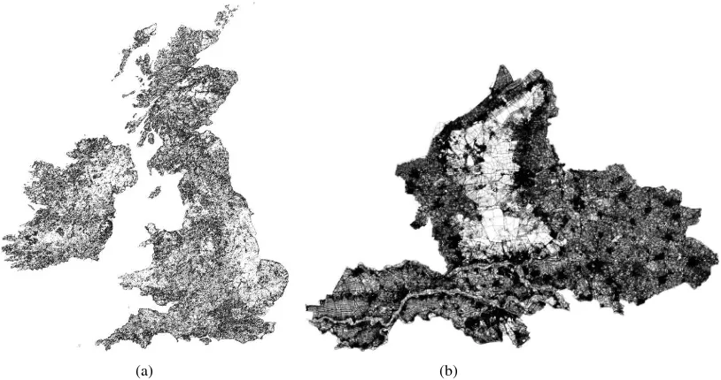
• CORINE Land Cover dataset for an area of the United King-dom and Ireland with approximately 100,000 faces and an area around Estonia with approximately 130,000 faces both intended to be used at a 1:100,000 map scale (Figure 5a).
• A road network dataset of the Netherlands (in Dutch: Na-tionaal Wegen Bestand). This dataset is intended for use at a 1:25,000 map scale. Note that the cycles/ areas of the road network (i. e. the ‘space between the roads’) have been used for creating a planar area partition and driving the general-ization procedure (iteratively picking the smallest cycle of the road network to be removed, ultimately leading to re-moval of an road from the network, as described by ˇSuba et al. (2014b)). It contains approximately 200,000 of these areas.
20x 60x 100x 160x 220x Smallest field size (as average object size)
0.0 0.1 0.2 0.3 0.4 0.5 0.6 0.7 0.8
Runtime (h)
cadastral land cover Estonia land cover UK
Figure 6: Processing time needed versus field size (smallest fields). Note that the smallest field size was determined based on the average feature size in the dataset.
All datasets have been processed in parallel (multiple fields at same time) at our research server with 16 CPU cores1. All vario-scale tables are stored in a PostgreSQL database management system extended with PostGIS2.
The different datasets we processed show that the approach works, even for different types of input data (land cover data, road net-work and cadastral map). The successful processing with the road network dataset demonstrates that when it is important to have neighbouring features available (for generalization decisions), it is possible to shrink the domain inwards. With this approach we are still able to process fields in parallel, while each feature is just processed once.
To obtain insights in what is a reasonable field size for the small-est fields in the fieldtree, we run the whole process (constructing fieldtree, distributing the objects, generalization field by field, fi-nalization) with different sizes for the smallest fields in the field-tree. We varied the sizes of these fields, based on the average size of a feature in the dataset. We used sizes varying from 20 to 160 times the average feature size. Figure 6 shows the resulting tim-ings we obtained. The graph shows that as rule of thumb, we can set the size of smallest fields to 100 times the average feature size (i. e. around 10,000 objects in the smallest fields) and that the to-tal runtime is then rather optimal. Furthermore, this graph learns us that too small fields lead to a lot of overhead in processing: Many tables that contain a little bit of data, and cannot be gen-eralized sufficiently for the next level (so no reduction will take place at a level, so waste of processing time / overhead in terms of copying data to the next level).
For the biggest dataset (the cadastral map with 880,000 faces) we investigated in-depth the runtime needed for the generalization step. In a sequential run this step took 7900 seconds (slightly more than 2 hours). We measured the time needed for parallel processing field by field. We also investigated whether this could be shortened, by taking a different order of processing the fields.
1
HP DL380p Gen8 server (with two 8-core Intel Xeon processors, E5-2690 at 2.9 GHz, 128 GB main memory, and RHEL 6 operating system) with Disk storage (direct attached) with 400 GB SSD, 5 TB SAS 15K rpm in RAID 5 configuration (internal), and 2 x 41 TB SATA 7200 rpm in RAID 5 configuration.
2
PostgreSQL 9.3.4 and PostGIS 2.2.0dev
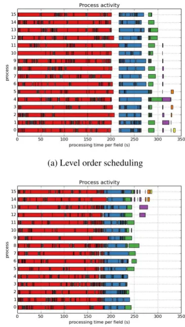
(a) Level order scheduling
(b) Parent child scheduling
Figure 7: Two different scheduling orders for the cadastral dataset. Every rectangle represents one field. Note that different colours correspond to the levels of the fieldtree (i. e. red corre-sponds to the fields with finest grid size). (a) Level order schedul-ing. The process waits until all fields of the same level are pro-cessed before processing of the next level starts. (b) The parent child scheduling. Fields are scheduled for processing when all its upto 9 child fields are done.
Figure 7 shows two possible scheduling strategies for distributing work in multiple parallel CPUs.
The first strategy, the ‘level order’ scheduling, takes care of all fields at the same level before the higher level is started. The second and more refined strategy, the ‘parent child’ scheduling, will schedule the parent field for scheduling if all its children are processed.
It is clear that parallel processing significantly speeds up the whole process, run time is shortened with a factor between 7900
340 = 23
and 7900290 = 27. Given the 16 CPUs the speed up lies between factor 7900
340∗16= 1.4and
7900
290∗16= 1.7in our implementation.
(a) (b)
Figure 5: Two of the testing datasets: (a) CORINE and (b) cadastral map
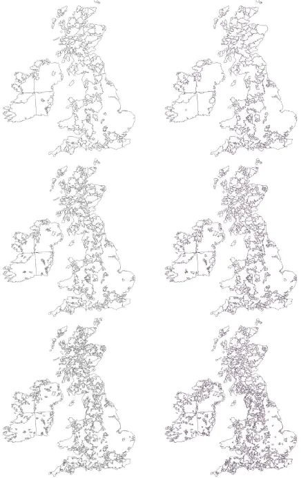
As last, we found having processed the CORINE land cover dataset the majority of the generalization work was performed at the end of the whole process (40% of the runtime was devoted to process-ing the last field). After inspection, this turned out to be caused by some very large polygons remaining to the end of the pro-cess (these massive polygons with a lot of holes representing the land between all small settlements only fitted in the very last field of the Fieldtree). Apart from having a negative influence on the run time, these polygons will also have a negative impact on the cartographic result as these polygons will keep their full original amount of detail until when they are processed. In order to assess the visual impact, we compared the result of the parallel version of the algorithm with the sequential run (original non-parallel ap-proach); see Figure 8. The visual impression of both approaches are quite similar. The main differences are that the amount of ver-tices is higher in the parallel version (counting showed that this is roughly twice the amount of vertices).
6. CONCLUSIONS AND FUTURE WORKS
An approach for automated map generalization to obtain a vario-scale data structure of massive datasets has been proposed and tested. We have described all steps of the process chain which we apply and we tested the approach with real data. It has been shown that our approach is generic and works for different types of input data such as land cover or road network data. We have tested with real world data and got significant speed ups (upto factor 27 on 16 core machine), although we still plan to test the approach with a really massive dataset (e. g. topographic dataset of The Netherlands or CORINE for whole of Europe) which not fitting in main memory. We expect that larger dataset will ben-efit from having even more parallelism assuming the hardware is there; for example 32 processes. The design is scalable: each job gets its input data from the database and writes the output again to the database. So, the whole dataset does not have to fit in main memory, as long as the active jobs do fit in memory, the process should remain efficient. We have to explore this further. In case we keep the same amount of main memory but increase the number of parallel processes, will these jobs still fit in main memory. If not, we should either make average job size smaller or add more memory.
The Fieldtree is very appropriate as it is good start for divide-and-conquer, but also offers very useful multiple levels: What is not solved at lowest level can be solved at higher level (which is also glueing partial solutions of lower level fields together). This fits very well with our approach to map generalization, but the divide-and-conquer approach using the Fieldtree may not be limited to map generalization only (and other spatial problems could benefit from this type of organization as well, e. g. obtaining an explicit topological data structure).
We have presented two approaches for scheduling the parallel work. We are aware of the fact that both of the scheduling ap-proaches are still sub-optimal. An improved scheduling might be based on processing the largest fields (with respect to number of features contained) first and smaller later, and applying dynamic scheduling from a ‘work-pool’.
Furthermore, we only carried out limited evaluation of the car-tographic end results and as we found out with processing the CORINE land cover dataset with massive polygons, our approach is less robust against these polygons.
This shows that there are still some open questions to be an-swered. Our future work includes:
• Very large features survive until the end and are not gener-alized. These large objects and also their island objects are affected. In our tests typical cases are: large ‘background’ polygons, or very long infrastructure features, such as rivers and roads. Our proposal for a solution in this case: split the large features. This raises another interesting challenge: How to best split these large features into smaller (artificial) chunks.
The size of fields is reflected in generalization quality. If the fields are big the ‘seams’ of the field may be visible, because the objects on the boundary could not be generalised for a long time while the rest of the field has been simplified a lot. Contrary, too small fields will contain less object which leads to less generalization options again leading to a worse result.
• The Fieldtree subdivides space regularly where the density of the original data is not considered. In some cases a large city is in one field (lot of generalization processing is needed) while the rest of the fields cover the rural regions where not much simplification is required. Then most of the re-sources are spent on the field containing the city while the other fields are already processed. A good strategy would be to locally deepen the fields at lowest level where high data density regions are reached. This would result in a slightly different Fieldtree: a structure of which the lowest deepened fields are not covering the whole domain anymore.
• Assessing the cartographic quality of our parallel creation of the vario-scale structure compared to the traditional cre-ation (based on global criterion for least important feature). For example is it possible to see the seams of the Fieldtree that subdivide the work? This is not expected so much, but should be verified with user tests.
• As the parallel creation is not based anymore of the global criterion (of least important feature), the Fieldtree structure can be also used for the update of vario-scale structures: only the field with updated data needs to be reprocessed, and if generalized result of field is rather different, then also the parent(s) needs to be reprocessed (recursively).
ACKNOWLEDGEMENTS
This research was supported by: (i) the Dutch Technology Foun-dation STW, which is part of the Netherlands Organisation for Scientific Research (NWO), and which is partly funded by the Ministry of Economic Affairs (project code 11185); (ii) the Eu-ropean Location Framework (ELF) project, EC ICT PSP Grant Agreement No. 325140.
References
Armstrong, M. P. and Densham, P. J., 1992. Domain decompo-sition for parallel processing of spatial problems. Computers, Environment and Urban Systems 16(6), pp. 497 – 513.
Dean, J. and Ghemawat, S., 2004. MapReduce: Simplified Data Processing on Large Clusters. In: Proceedings of the 6th Con-ference on Symposium on Opearting Systems Design & Imple-mentation - Volume 6, OSDI’04, USENIX Association, Berke-ley, CA, USA, pp. 10–10.
Ding, Y. and Densham, P. J., 1996. Spatial strategies for parallel spatial modelling. International journal of geographical infor-mation systems 10(6), pp. 669–698.
Eldawy, A., Li, Y., Mokbel, M. F. and Janardan, R., 2013. Cg hadoop: Computational geometry in mapreduce. In: Pro-ceedings of the 21st ACM SIGSPATIAL International Con-ference on Advances in Geographic Information Systems, SIGSPATIAL’13, ACM, New York, NY, USA, pp. 294–303.
Frank, A. U. and Barrera, R., 1990. The Fieldtree: A data struc-ture for Geographic Information Systems. In: Proceedings of the First Symposium on Design and Implementation of Large Spatial Databases, SSD ’90, Springer-Verlag New York, Inc., New York, NY, USA, pp. 29–44.
Guan, X., Wu, H. and Li, L., 2012. A Parallel Framework for Processing Massive Spatial Data with a Split-and-Merge Paradigm. Transactions in GIS 16(6), pp. 829–843.
Hawick, K. A., Coddington, P. D. and James, H. A., 2003. Distributed frameworks and parallel algorithms for process-ing large-scale geographic data. Parallel Computprocess-ing 29(10), pp. 1297–1333.
Huang, L., Meijers, M., ˇSuba, R. and van Oosterom, P., 2014. En-gineering web maps with gradual content zoom and streaming transmission of refinements for vector data display at arbitrary map scale. Submitted to ISPRS Journal of Photogrammetry and Remote Sensing (December 11, 2014).
Meijers, M. and Ledoux, H., 2013. EdgeCrack: a parallel Divide-and-Conquer algorithm for building a topological data struc-ture. In: C. Ellul, S. Zlatanova, M. Rumor and R. Laurini (eds), Urban and Regional Data Management: Annual 2013, CRC Press, pp. 107–116.
Meng, L., Huang, C., Zhao, C. and Lin, Z., 2007. An improved Hilbert curve for parallel spatial data partitioning. Geo-spatial Information Science 10(4), pp. 282–286.
Sharker, M. H. and Karimi, H. A., 2014. Big Data. CRC Press, chapter Distributed and Parallel Computing, pp. 1–30.
Stoter, J., Post, M., van Altena, V., Nijhuis, R. and Bruns, B., 2014. Fully automated generalization of a 1:50k map from 1:10k data. Cartography and Geographic Information Science 41(1), pp. 1–13.
Thiemann, F., Warneke, H., Sester, M. and Lipeck, U., 2011. A Scalable Approach for Generalization of Land Cover Data. In: S. Geertman, W. Reinhardt and F. Toppen (eds), Advancing Geoinformation Science for a Changing World, Lecture Notes in Geoinformation and Cartography, Springer Berlin Heidel-berg, pp. 399–420.
van Oosterom, P., 2005. Variable-scale Topological Data Struc-tures Suitable for Progressive Data Transfer: The GAP-face Tree and GAP-edge Forest. Cartography and Geographic In-formation Science 32(11), pp. 331–346.
van Oosterom, P. and Vijlbrief, T., 1996. The Spatial Location Code. In: Proceedings of the 7th International Symposium on Spatial Data Handling, SDH’96.
van Oosterom, P., Meijers, M., Stoter, J. and ˇSuba, R., 2014. In: D. Burghardt, C. Duchene and W. Mackaness (eds), Abstract-ing Geographic Information in a Data Rich World: Methodolo-gies and Applications of Map Generalisation, Lecture Notes in Geoinformation and Cartography, Springer, chapter Data Structures for Continuous Generalisation: tGAP and SSC, pp. 83–118.
van Putten, J. and van Oosterom, P., 1998. New results with Generalized Area Partitionings. In: Proceedings of the In-ternational Symposium on Spatial Data Handling, SDH’98, pp. 485–495.
ˇSuba, R., Meijers, M., Huang, L. and van Oosterom, P., 2014a. An area merge operation for smooth zooming. In: J. Huerta, S. Schade and C. Granell (eds), Connecting a Digital Europe Through Location and Place, Springer Lecture Notes in Geoin-formation and Cartography, Springer International Publishing, pp. 275–293.
Wang, H., Fu, X., Wang, G., Li, T. and Gao, J., 2011. A com-mon parallel computing framework for modeling hydrological processes of river basins. Parallel Computing 37(67), pp. 302 – 315.