STATISTIC TESTS AIDED MULTI-SOURCE DEM FUSION
C. Y. Fu a, J. R. Tsay a *
a Dept. of Geomatics, National Cheng Kung University, No.1, University Road, Tainan, Taiwan - (P66044099, tsayjr)@mail.ncku.edu.tw
Youth Forum
KEY WORDS: DEM Fusion, Blunder Detection, Statistic Test
ABSTRACT:
Since the land surface has been changing naturally or manually, DEMs have to be updated continually to satisfy applications using the latest DEM at present. However, the cost of wide-area DEM production is too high. DEMs, which cover the same area but have differentquality, grid sizes, generation time or production methods, are called as multi-source DEMs. It provides a solution to fuse multi-source DEMs for low cost DEM updating. The coverage of DEM has to be classified according to slope and visibility in advance, because the precisions of DEM grid points in different areaswith different slopes and visibilities are not the same. Next, difference DEM (dDEM) is computed by subtracting two DEMs. It is assumed that dDEM, which only contains random error, obeys normal distribution. Therefore, student test is implemented for blunder detection and three kinds of rejected grid points are generated. First kind of rejected grid points is blunder points and has to be eliminated. Another one is the ones in change areas, where the latest data are regarded astheirfusion result. Moreover, the DEM grid points of type I error are correct data and have to be reserved for fusion. The experiment result shows that using DEMs with terrain classification can obtain better blunder detection result. A proper setting of significant levels (α) can detect real blunders without creating too many type I errors. Weighting averaging is chosen as DEM fusion algorithm. The priori precisions estimated by our national DEM production guidelineare applied todefine weights.
Fisher’s test is implemented to prove that the priori precisions correspond to the RMSEs of blunder detection result.
* Corresponding author
1. INTRODUCTION
1.1 Background
Nowadays, DEMs (Digital Elevation Models) are useful data which are applied in many fields, such as urban planning, disaster prevention and engineering. Therefore, the quality of the DEM decides its applicability. However, the earth surface has been changing by endogenetic process, exogenetic process and manual development. If the DEM is not updated continually, the elevation data will be inconsistent with the real situation. So far, aero-photogrammetry, airborne LiDAR (Light Detection And Ranging) and satellite based sensors are main methods for wide-area DEM generation, but their costsare too high for DEM updating.
The purpose of data fusion is to combine the advantages of different data sources and thus provide a better one. Take image fusion for example, a panchromatic image and a multispectral image are fused to derive a pan-sharpening one with higher spatial and spectral resolutions. For the same reason, if multiple DEMs which cover the same region are fused together, the result will disregard the bad data and obtain the better ones. Since the quality, grid sizes, generation time and production methods of these DEMs are often different, they are also known as source DEMs, and it provides a solution to fuse multi-source DEMs for lower cost DEM updating.
1.2 Literature Review about DEM Fusion
Weighting averaging is a common method for DEM fusion. Papasaika et al. (2008) and Papasaika and Baltsavias (2009)
derived the residual map by subtracting two DEMs. Then, the residual map and geomorphological indexes (slope, aspect and roughness) were used to determine weight in each grid. DEMs produced by stereo pairs, LiDAR and InSAR (Interferometry Synthetic Aperture Radar) are often averaged together (Roth et al., 2002;Podobnikar, 2005;Reinartz et al., 2005;Hoja et al., 2006;Hoja and d’Angelo, 2009;Choussiafis et al., 2012;Jain et al., 2014).
Another fusion approach is to generate an initial approximate terrain surface. Then, DEMs are added incrementally to reform the approximate surface. Approximate surface can be created by DEM with the biggest grid size (Chen et al., 2012), linear prediction (Kraus and Pfeifer, 2001) or the lowest point (Axelsson, 2000 ; Sohn and Dowman, 2002). Sparse representation (Papasaika et al., 2011;Schindler et al., 2011) constructs an ideal terrain surface from high accurate DEMs. Since the residuals between original DEMs and ideal terrain should be the smallest, least squaresadjustment is implemented to derive themost probable valuesof each DEM.
Schultz et al. (1999;2002) and Stolle et al. (2005) adopted self-consistency for processing DEMs generated from different stereo pairs in the same project to eliminate blunders. Next, all DEMs without blunders are fused to obtain a better result. Fusing DEM in frequency domain is a concept which was firstly introduced by Honikel in 1998 and was tested by other researches (Crosetto and Aragues, 2000;Karkee et al., 2008). Combining data from stereo pairs, LiDAR and InSAR to interpolate a better DEM is another DEM fusion method, which
integrates the advantages of different data sources (Crosetto and Crippa, 1998; Hosford et al., 2003).
1.3 Purpose
The purpose of the research is to fuse multi-source DEMs to derive a fusion result with better quality. The word “better quality” in this paper is defined that the number of blunders and the influence of random errors in original DEMs are decreased after DEM fusion. To avoid complicated discussion, only two DEMs are used for blunder detection, and weighting averaging is conducted to reduce the random errors.
2. METHODOLOGY
2.1 DEM Registration
Data pre-processing has to be done before fusion because the coordinate datum and formats of DEMs are usually inconsistent
with one another’s. First up, the horizontal and vertical datums of all DEMs are transformed into the same horizontal and vertical ones, respectively. Then, if the grid sizes are different, DEMs with higher resolution will be resampled into the same resolution of DEM with the largest grid size.
2.2 Terrain Classification
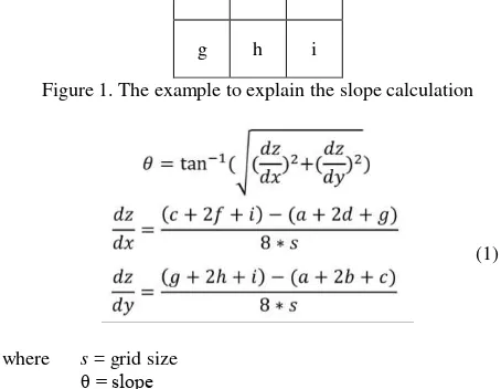
According to DEM production guidelines from MOI (Ministry of the Interior), Taiwan (2003), the precision of DEM is highly related to the slope and visibility (=100% - percentage of tree coverage) of the terrain surface. As long as the slope increases or the visibility decreases, the quality of corresponding DEM datawill become worse. Therefore, it is necessary to classify the terrain by the slope and visibility. The calculation of slope is shown below (Burrough and McDonnell, 1998):
a b c
d e f
g h i
Figure 1. The example to explain the slope calculation
(1)
where s = grid size
θ = slope
Orthoimages, which have the same coverage and generation periods as DEMs, are used for visibility classification. However, since the relief displacements in orthoimages are not totally removed, the invisible regions are often classified inaccurately. Therefore, stereo pairs of aerial images are introduced for visibility classification in manual manner on stereo models.
2.3 Blunder detection
Blunder detection is the most important part of fusion in this paper. Although the magnitudes of gross errors will be reduced after fusion, the blunders may still existin the result (Schultz et al., 2002). In other word, the fusion result is still wrongunless the blunders are removed. Strictly speaking, systematic errors have to be detected and totally corrected before fusion. In fact, however, there are different kinds of systematic errors in DEM and theircombination is too complicated to correct. Hence, this paper does not discuss the correction of systematic errors.
First step of blunder detection is that one subtracts a DEM from another one to obtain a difference DEM (dDEM). Then, a statistic test is used to find the gross errors. If the DEM contains only random errors, the elevations will obey normal distribution, and the elevation difference will also obey normal distribution, according to the law of error propagation (Schultz et al., 1999; Schultz et al., 2002;Stolle et al., 2005). Therefore, a null hypothesis assumes that all values in dDEM obey normal distribution:
H0 : dh ~ N(0, dh) dh (2)
where dh = elevation difference
dh= the STD of elevation difference
Then, student test is utilized with a proper significant level α. The statistic test will be done iteratively until there is no rejected grid point any more. The rejected grids include blunders, change area or type I error. Blunders have to be eliminated while the correct observations are remained. In change areas, the elevations are changed naturally or manually during the period. Hence, the latest data are regarded as the fusion result. Type I errors mean the data are correct, but they are misunderstood as blunders. Therefore, these grids have to be reserved for fusion. In this paper, stereo measuring is applied to distinguish whether the rejected grids are blunders, change areas or type I errors.
2.4 Weighting Averaging
In this paper, weighting averaging is used for DEM fusion, so deciding weights becomes an important issue. Using the precisions of DEM data to define their weights is an intelligent approach (Fuss, 2013). Therefore, a lot of studies aim to estimate DEM precision. Using geomorphological index is a popular method (Podobnikar, 2005;Papasaika, et al, 2008; Papasaika and Baltsavias, 2009). Another method is to generate residual map of DEMs (Kraus & Pfeifer, 2001;Roth et al, 2002;Papasaika, et al, 2008;Papasaika and Baltsavias, 2009). However, theafore-mentionedmethods determine the precision at each grid point, so the cost of fusion becomes very high. Since the priori precisions of DEMs measured in different terrain surface are estimated according to the national guidelines published by MOI (2003), grids in the sameclass of terrain surface are fused by the same weight. The relation between precision and weightingvalue is expressed below:
(3)
where WDEM = the weight of DEM σ2
DEM = the variance of DEM
3. STUDY AREA AND DATA INFORMATION
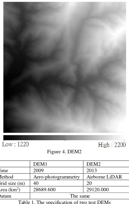
Mountain area around Kaohsiung and Pingtung, Taiwan is chosen as the study area. Figure 2 shows the ortho images in the study area in different periods. Since a serious typhoon hit Taiwan in 2009, the land surface had been changed a lot and become fragile while raining. However, there is no obvious land surface changing from 2009 to 2013. Two DEMs are selected for this experiment and are displayed in figure 3 and figure 4. Their specification is expressed in table 1.
(a) (b) (c)
Figure 2. The orthoimages in the study area (a) Before typhoon (b) In 2009 (c) In 2013
Figure 3. DEM1
Figure 4. DEM2
DEM1 DEM2
Time 2009 2013
Method Aero-photogrammetry Airborne LiDAR
Grid size (m) 40 20
Area (km2) 28689.600 29120.000
Datum The same
Table 1. The specification of two test DEMs
4. EXPERIMENT RESULT AND ANALYSIS
4.1 DEMRegistration Result
Datum transformation is not needed because two DEMs have the same horizontal and vertical coordinate systems, but have different grid sizes. In this paper, the small grid DEM is adjusted to be consistent with the big one rather than using big grid DEM to interpolate into small one. The reason is that there is no algorithm which interpolates terrain data without additional errors except for random one (Fisher and Tate, 2006; Wechsler, 2007). Hence, DEM2 only reserves the grids whose horizontal coordinates are the same as coordinates of DEM1, and this approach generates no additional error due to resampling. The process of resampling is illustratedin figure 5. Besides, the coverage areas of two DEMs are different, so the boundaries of two DEMs must be aligned.
Figure 5. The process of resampling
4.2 Terrain Classification Result
The slope is classified into three groups: low (< 15ᵒ), middle (15ᵒ≤ θ < 45ᵒ), and high (≥ 45ᵒ) (MOI, 2003). Figure 6 shows the slope map of the study area. Most grids belong to middle slope. The study area is classified into low visibility (< 50%) and high visibility (≥ 50%). Since there is no obvious land surface changing, the change area is not taken into account in this step. Therefore, six classification labels are derived by combining three kinds of slope and two types of visibility. Table 2 display the classification labels. The classification map is displayed in figure 7. The number of grids of each label is shown in table 3.
Figure 6. The slope map
high visibility
(≥ 50%) low visibility (< 50%) low slope (< 15ᵒ) Label 1 Label 4
middle slope (15ᵒ≤ θ < 45ᵒ)
Label 2 Label 5
high slope (≥ 45ᵒ
Table 2. Six labels and classification criteria
Label Number % Label Number %
1 776 4.33 4 212 1.18
2 5812 32.41 5 9344 52.11
3 1189 6.63 6 598 3.34
Number of total grids 17931
Table 3. The percentage of each label
Figure 7. The classification map
4.3 Blunder Detection Result
Two discussions are introduced below. One is to choose proper significant levels (α) for blunder detection. Grids in different label have to be conducted blunder detection individually because the precision of each labels is different from one another. The other one is to prove that the result of blunder detection with classified data is better than DEM without classification.
4.3.1 Determine α
Since α influences the number of type I errors and type II errors, it is necessary to determine proper α values before blunder detection. Three cases with different α setting are introduced. In case 1, α is set as 0.1% while α in case 2 is 0.5%. Case 3 combines the advantages of former cases and is the best of the three. Although RMSE is a common index to evaluate the precision of DEM, it will become unreliable as long as data do not obey normal distribution (Fisher and Tate, 2006). The rejection ratio is used for analysis and, if needed, the related DEM points are checked on stereo models. The RMSEs of three cases after detection are expressed in table 4, and the ratio of rejected grids in each case is illustratedin table 5.
The RMSEs of label 1 are very small in all cases, but the rejected ratios of grids are up to 52.84% and 93.69%. After stereo measuring, the elevations in 2013 are actually lower than those in 2009. Therefore, grids in label 1 are regarded as change areas and only data in DEM 2 are reserved. Since case 2 is able to detect more change areas than case 1, α in label 1 is set as
In label 2 and label 6, though the rejection ratios increase when the α becomes bigger, the RMSEs do not decrease obviously. Therefore, the DEM points which are rejected in case 2 but pass the statistic test in case 1, belong to the ones of type I errors, so the values of α in label 2 and label 6 are set as 0.1%.
In other labels, as the α increase, the RMSEs become smaller, but the rejection ratios become too high. Stereo measurement is applied to find the reason. Most DEM points belong to the ones of type I errors, so the values of α in label 3, label 4 and label 5 are setto0.1%. Some rejectedDEM points, which belong to the ones of type I errors, are located at the boundary of different labels, so these type I errors result from inaccurate classification. As long as the classification is improved, this kind of type I error willbe reduced.
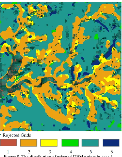
To sum up, α is 0.5% in label 1 can detect most of the change areas, while α is 0.1% in other labels is able to reject real blunders without creating too many type I errors. Case 3 follows this setting and the result of case 3 is used for fusion. Figure 8 shows the result of case 3.
Table 4. The RMSEs ofthree cases
Case 1 Case 2 Case 3
Table 5. The ratio of rejected DEM points in each case
Figure 8. The distribution of rejected DEM points in case 3
4.3.2 Blunder Detection with and without Classification
In this section, DEM blunders are detected by using dDEMs with and without classification, respectively. Table 6 displays the RMSEs and table 7 shows the rejection ratios. Since over
Table 6. The RMSEs with and without classification
Label α (%) With classification
Without classification Rejection ratio (%) Rejection ratio (%)
1 0.5 93.69
Table 7. The rejection ratio with and without classification
4.4 DEM Fusion
The priori precision in each label is estimated by Eq. (3) according to our national production guidelines (MOI, 2003) and the results are shown in table 8:
(3)
where σ= The estimated priori precision of DEM
a= The precision of measurement
b = The term caused byslope c = a constant for t
t = The average tree height
DEM 1
Label Precision (m) Label Precision (m)
1 0.8 4 4.8
2 1.5 5 5.5
3 6.5 6 10.5
DEM 2
Label Precision (m) Label Precision (m)
1 0.5 4 10.5
2 0.8 5 10.8
3 1.3 6 11.3
Table 8. The estimated priori precision in each label
According to the law of error propagation, the variance of dDEM equals to the sum of variances of DEM 1 and DEM 2:
(4)
Therefore, the RMSEs of dDEM are used to test whether the priori precisions are proper or not. The null hypothesis is assumed as followsand fisher’s test is applied:
(5)
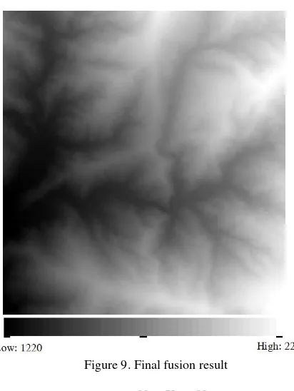
The fisher’s test is not done for those DEM grid points of label 1 because label 1 area is regarded as change area and DEM2 data is the fusion results in label 1 area. Since all of the other grid points pass the fisher’s test, the prior precisions are applied then for weighting averaging. The final fusion result is illustrated in figure 9.
Figure 9. Final fusion result
5. CONCLUSIONS
In this paper, a procedure of multi-source DEM fusion is introduced. The fusion result is better than original DEMs because the blunders are detected and eliminated by statistic tests. The terrain surface has to be classified by slope and visibility. Otherwise, over 99% of DEM grid points will be rejected after blunder detection. Three kinds of grid points are rejected in blunder detection. Real blunders have to be eliminated. Change areas are also rejected by statistic test. Only data measured after changing can be fused. In the experiment, all grid points in label 1 had been changed, so their DEM2 data are regarded as the fusion result. The other one is type I error. Those grid points with normal measurements have to join DEM fusion. The value of α is 0.1% in all labels except label 1. The maximal RMSE of dDEM after blunder detection is 18.2 m in the regions with high slope and low visibility. Since all the RMSEs of dDEM correspond to the priori precisions, the weights are determined and the fusion result is derived by weighting averaging.
REFERENCES
Axelsson, P., 2000. DEM generation form laser scanner data using adaptive TIN models. International Archives of Photogrammetry and Remote Sensing, Vol. 33(Part B4), pp. 110-117.
Burrough, P. A. and McDonnell, R. A., 1998. Principles of Geographical Information Systems. Oxford University Press, p. 190.
Chen, Z., Devereux, B., Gao, B., and Amable, G., 2012. Upward-Fusion Urban DTM Generating Method Using Airborne Lidar Data, ISPRS Journal of Photogrammetry and Remote Sensing, Vol. 72, pp. 121–130
Choussiafis, C., Karathanassi, V., and Nikolakopoulos, K., 2012. Mosaic Methods for Improving the Accuracy of Interferometric Based Digital Elevation Models. Proceedings of
Crosetto, M. and Aragues, F. P. 2000. Radargrammetry and SAR interferometry for DEM generation: Validation and data fusion. CEOS SAR Workshop, Vol. 450, pp. 367-372.
Crosetto, M. and Crippa, B., 1998. Optical and radar data fusion for DEM generation, International Archives of Photogrammetry and Remote Sensing, Vol. 32(4), ISPRS Commission IV Symposium on GIS – Between Visions and Applications, Stuttgart, Germany, pp. 128–134.
Fisher, P. F. and Tate, N. J. 2006. Causes and consequences of error in digital elevation models. Progress in Physical Geography, Vol. 30(4), pp. 467–489.
Fuss, C. E., 2013. Digital elevation model generation and fusion.
Master’s thesis, The University of Guelph, Ontario, Canada.
Hoja, D., Reinartz, P., and Schroeder, M., 2006. Comparison of DEM generation and combination methods using high resolution optical stereo imagery and interferometric SAR data, In ISPRS (Ed.), ISPRS Commission I Symposium, Vol. 36 Paris, Marne la Vallee, France.
Hoja, D. and d’Angelo, P., 2009. Analysis of DEM combination methods using high resolution optical stereo imagery and interferometric SAR data, In ISPRS Hannover Workshop 2009.
Honikel, M. 1998. Fusion of optical and radar digital elevation models in the spatial frequency domain. Second International Workshop on Retrieval of Bio- & Geo-Physical Parameters from SAR Data for Land Applications, Vol. 441, pp. 537-543.
Hosford, S., Baghdadi, N., Bourgine, B., Daniels, P., and King, C., 2003. Fusion of airborne laser altimeter and RADARSAT data for DEM generation, In IEEE International Geoscience and Remote Sensing Symposium, Vol. 2, pp. 806–808.
Jain, M., Deo, R., Kumar, V., and Rao, Y. S., 2014. Evaluation of Time Series TanDEM-X Digital Elevation Models, The International Archives of the Photogrammetry, Remote Sensing and Spatial Information Sciences, Vol. XL-8, pp. 437-441.
Karkee, M., Steward, B. L., and Aziz, S. A. 2008. Improving quality of public domain digital elevation models through data fusion. Biosystems Engineering, Vol. 101(3), pp. 293-305.
Kraus, K. and Pfeifer, N., 2001. Advanced DTM Generation from Lidar Data. International Archives of Photogrammetry and Remote Sensing, Vol. 34, pp. 22-24.
MOI (Ministry of the Interior), Taiwan, 2003. National Guidelines for Production of High Accuracy and High Resolution Digital Terrain Models.
Papasaika, H., Poli, D., and Baltsavias, E., 2008. A framework for the fusion of digital elevation models. Int Arch Photogramm Remote Sens, pp. 811-818.
Papasaika, H. and Baltsavias, E., 2009. Fusion of LiDAR and photogrammetric generated digital elevation models. Proceedings of the ISPRS Hannover Workshop on High-Resolution Earth Imaging for Geospatial Information, Hannover, Germany.
Papasaika, H., Kokiopoulou, E., Batsavias, E., Schindler, K., and Kressner, D., 2011. Fusion of Digital Elevation Models using Sparse Representations, Proceedings of the 2011 ISPRS
Conference on Photogrammetric Image Analysis, PIA’11, pp. 171–184. Berlin, Heidelberg: Springer-Verlag.
Podobnikar, T., 2005. Production of integrated digital terrain model from multiple datasets of different quality. International Journal of Geographical Information Science, Vol. 19(1), pp. 69-89.
Reinartz, P., Müller, R., Hoja, D., Lehner, M., and Schroeder, M., 2005. Comparison and Fusion of DEM Derived from SPOT-5 HRS and SRTM Data and Estimation of Forest Heights, EARSEL Workshop on 3D-Remote Sensing, Portugal (on CD-ROM).
Roth, A., Knopfle, W., Strunz, G., Lehner, M., and Reinartz, P., 2002. Towards a global elevation product: combination of multi-source digital elevation models. International Archives of Photogrammetry Remote Sensing and Spatial Information Sciences, Vol. 34(4), pp. 675-679.
Schindler, K., Papasaika-Hanusch, H., Schuetz, S., and Baltsavias, E., 2011. Improving Wide-Area DEMs Through Data Fusion – Chances and Limits, ETH Publications, pp. 159-170.
Schultz, H., Riseman, E.M., Stolle, F.R., and Woo, D. -M., 1999. Error Detection and DEM Fusion Using Self-Consistency, The Proceedings of the Seventh IEEE International Conference on Computer Vision, pp. 1174-1181.
Schultz, H., Hanson, A., Riseman, E. M., Stolle, F. R., Zhu, Z., and Woo, D.-M., 2002. A Self-consistency Technique for fusing 3D Information, IEEE Fifth International Conference on Information Fusion, Annapolis Maryland, pp. 1106-1112.
Sohn, G. and Dowman, I. J., 2002. Terrain surface reconstruction by the use of tetrahedron model with the MDL criterion. International Archives of Photogrammetry Remote Sensing and Spatial Information Sciences, Vol. 34(3/A), pp. 336-344.
Stolle, F., Schultz, H., and Woo, D. -M., 2005. High-resolution DEM generation using self-consistency. In ISPRS Hannover
Workshop 2005 on “High-Resolution Earth Imaging for
Geospatial Information”, Hannover.
Wechsler, S. P. 2007. Uncertainties associated with digital elevation models for hydrologic applications: a review. Hydrology and Earth System Sciences, Vol. 11, pp. 1481–1500.