FOREST SPECIES CLASSIFICATION BASED ON STATISTICAL POINT PATTERN
ANALYSIS USING AIRBORNE LIDAR DATA
J. Li a, *, B. Hu a, T. L. Noland b
a Dept. of Earth and Space Science and Engineering, York University, Toronto, ON, M3J1P3, Canada - (ljili, baoxin)@yorku.ca
b Ontario Ministry of Natural Resources, 1235 Queen St. East, Sault Ste. Marie, ON, P6A 2E5, Canada - [email protected]
Commission VI, WG VI/4
KEY WORDS: Remote Sensing, LiDAR, Point Pattern Analysis, K-function, PCA, Classification
ABSTRACT:
The paper investigated the effectiveness of point pattern methods in the application of forest species classification using airborne LiDAR data. The forest stands and individual trees in our study area were classified as either shade tolerant or intolerant species. The purpose of adopting the point pattern methods is to develop new features to effectively characterize the pattern of internal foliage distribution of forest stands or individual trees. Three methods including Quadrat Count, Ripley’s K-function, and Delaunay Triangulation were applied, and six feature groups were derived for a stand or tree sample. Feature selection was performed based on the derived features in order to find the best ones for the following classification procedure, which was implemented by two supervised and two unsupervised methods. These newly derived features were proved effective for the classification. The highest classification accuracy 97% was achieved at stand level and 90% at individual tree level. The sensitivity of classification accuracy to the number of features used was also investigated in this paper.
* Corresponding author. This is useful to know for communication with the appropriate person in cases with more than one author. 1. INTRODUCTION
The species type of natural forests plays important roles in the application of forest inventory and environment management. Trees in natural forests can be classified into certain categories on the basis of different physiological factors. The shade tolerance of a tree is generally used to indicate the tree’s capacity to develop, survive and grow beneath a forest canopy. Classifying the trees in forests into shade tolerance and intolerance is very important when forest and environment management decisions are made, for instance, providing enough sunlight conditions for maintaining intolerant species stands.
Conventionally, classification of tolerant and intolerant species in forests is mainly performed by foresters in the field based on the virtually identified structural information below canopies such as live crown ratio and radial growth patterns (Craig 1982). It is also a challenging task to carry out the classification from the remotely sensed imagery because there is little information provided about the foliage structure below tree canopies. The development of LiDAR instruments provides a good opportunity to exploit the structural difference between tolerant and intolerant trees because of its capacity to penetrate canopy vertically.
Several studies have been carried out on classification of species at the stand or individual tree level using airborne LiDAR data on the basis of a number of derived structure features. Holmgren et al. (2008) classified Scots pine, Norway spruce and deciduous trees based on the features related to crown shape, height distributions, pulse type and intensity. Reitberger et al. (2008) used the LiDAR data to classify coniferous and deciduous trees, based on five salient features
representing outer tree geometry, geometrical tree structure and pulse width. Vauhkonen et al. (2009) used alpha shape metrics for tree species classification in Scandinavian test site comprising 92 individual trees. Woods et al. (2008) used height percentiles as a part of the structure features derived from forest stands to calculate volume, basal area, and biomass. In these researches, the trees or stands were subdivided vertically into certain layers based on height percentiles, and the features are mostly some general statistical values derived for each layer, such as total number of points, mean intensity value, proportion of the first return, and so on. However, one of the issues is that these statistical features sometime are not sufficient to characterize the spatial distribution of leaves and branches within crowns. For example, the same number of points at a height layer maybe corresponds to two different foliage distribution patterns: clumped and dispersed, due to the different structures of species. To investigate and further characterize how leaves and branches distribute spatially within certain height layer, we adopted point pattern methods in this study. Point pattern analysis is a common statistical technique for analyzing spatial distributions of points, and it has been used in many study fields, such as mathematics, ecology, and forestry (Dale 1999, Fortin 2005). One of the advantages of this technique is its capability of directly processing point data with relatively simple calculations.
Objectives of this study are: 1) to develop the features using point pattern methods to characterize the degree of foliage clumping of forest stands and individual trees; and 2) to classify the stands and individual trees into three species categories, i.e. intolerant-deciduous, intolerant-coniferous and tolerant-International Archives of the Photogrammetry, Remote Sensing and Spatial Information Sciences, Volume XXXVIII-5/W12, 2011
deciduous. The tolerant-coniferous species is not common in our study area, thus it was not included in this study.
2. STUDY AREA AND DATA
The study area selected is near Sault Ste. Marie, Ontario, Canada (463356N, 832518W) at elevations ranging from 300m to 410m above the mean sea level. Located in the Great Lakes-St. Lawrence forest region, the natural forests in the study area include many homogeneous stands where one species dominated most of the area. Three typical species, Aspen (Populus tremuloides Michx.), Jack pine (Pinus banksiana Lamb.) and Sugar maple (Acer saccharum Marsh.), were selected in the forest area representing the three categories intolerant-deciduous species, intolerant-coniferous species and tolerant-deciduous species, respectively. Corresponding to each species, 50 forest stands of size 20 m × 20 m and 30 individual trees were chosen for this study. The trees attain a height of 21-30 m depending on site fertility. The species information of between the highest point and the lowest point.
about 0.15 m. The point clouds of the 150 forest standsand 90 individual trees were manually cut out from the raw dataset.
3. METHODS
3.1 Feature extraction
This section will describe the methods that were developed to derive novel features characterizing the vertical and horizontal distribution of tree elements, such as braches, leaves, etc. These features can be used to identify tree species at both stand level and tree level.
Let’s denote the entire LiDAR point cloud of a forest stand or an individual tree as an object. The LiDAR point clouds of an any given object were firstly subdivided into n equal height intervals (denoted as h1, h2, …, and hn) and ordered from high to low elevation. The points within each height interval were then projected on the horizontal plane. In this way, the object can be modelled by n two-dimensional layers ordered from top canopy to terrain. In this study, the value of n was chosen as 20. For a stand, the size of each layer is 20 m × 20 m, and for an individual tree the size is determined by the bonding box of the entire tree points projected on horizontal 2D plane. For each
layer, the distribution of LiDAR points which represent the distribution of foliage of trees in the layer, can be regarded as from dispersed to clumped pattern, and it can be further characterized by the following point pattern analysis methods.
Quadrant Count
Introduced by Dale (1999) and Tariq (2004), the Quadrant Count method was used in this study mainly to describe to what degree the foliage clumped. Following the definition in the literature (Dale 1999), the LiDAR points of each layer was partitioned into m equal size sub regions which were called as quadrants. In each quadrant the number of points that occur was counted and the distribution of the quadrant counts was used as the indicator of the spatial pattern of the LiDAR points. There are several ways to construct the indicator and the variance-to-mean ratio (feature denoted as VTMR) was computed and used in this study. To explain in detail, given the point data of a layer, the mean can be calculated as the ratio of number of points in the layer and number of quadrants in the layer. Let xi be the
number of points in each quadrant and m be the number of quadrants of the layer, the variance can be calculated as:
2 the point pattern is clustered, random, or dispersed (Tariq 2004). For example, if VTMR=1, the pattern is random and if VTMR>1, the pattern is clustered. In this study, instead of comparing VTMR with 1, we interpreted the value of VTMR as the degree that the point patter clustered. Generally, comparing with a small VTMR, a larger VTMR indicates that the point pattern tends to be more clustered. In this study, the size of each quadrant is chosen empirically as 0.25m
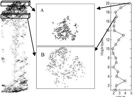
0.25m.Figure 1 shows the VTMR profile (right panel) of an aspen tree (left panel), and as examples, point clouds of two layers (middle panel). The two layers contained similar number of LiDAR points (385 of layer A vs. 419 of layer B), but they have different distribution patterns, represented by two different VTMR values: 4.9 for layer A and 2.6 for layer B. This is consistent with previous statement that larger VTMR value indicates the point pattern is more clumped, i.e. layer A is more clumped than layer B.
Figure 1. Left: point cloud of an aspen tree. Middle: projected point cloud of two example layers. Right: calculated VTMRs of the 20 height layers.
A
B
Ripley’s K-function
The method was mainly used in this study to describe where and at which scale the foliage clumped mostly. According to the definition proposed firstly by Ripley (1976) and further explained by Fortin (2005), if we denote as the density of LiDAR points in the area of an arbitrary 2D layer, the expected number of points occurring in a circle radius t centered on a
d as the distance between points i and j, the following statistic ˆ( ) randomness, the number of points in a circle follows a Poisson distribution and the expected value of K tˆ( )is 2
t
. An L-function is then created to characterize K-function’s deviations from its expected value (i.e. 2 point pattern is clumping at scale t.
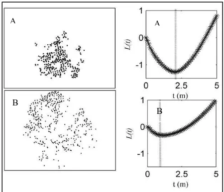
For a given layer of any object, the calculation of L tˆ( )resulted in a curve with certain positive or negative peaks. In the continuous steps, four features were extracted to characterize the L tˆ( )curve: the number of peaks determined by the number point pattern has larger positive peak values than the other layer B, and vice versa. In addition, as shown by the dash line on the two curve plots, the point cloud of layer A clumped with clumps at the distance scale about 2.1 m, while the point cloud of layer B clumped with clumps at the radius scale about 1.0 m.
Delaunay Triangulation
The Delaunay Triangulation method usually developed and applied for computational geometry (de Berg 2008); however, it is applied in this study to mainly characterize the distance distribution of the points. Given the LiDAR points projected in an arbitrary 2D layer, the delaunay triangulation was firstly created for the entire points in the layer. The edge length of the triangulations were then computed and sorted from short to long without repeat. The frequency distribution of the edge lengths was then computed. The variance of the frequency distribution (denoted as VarEdge) was then calculated and regarded as the feature extracted from the Delaunay Triangulation method. A large VarEdge value indicates the points are clumping, and a
smaller VarEdge value indicates the points are relatively less clumping.
Figure 2. The Lˆfunction derived from the LiDAR points of the two layers demonstrated in Figure 1. The dash line indicates the location of the radius scale t (Tpeak) where the points tend to be clumped to the maximum degree.
3.2 Feature selection
Generally, the features extracted from original dataset are not suggested to be used directly for classification or pattern recognition because not all of the features are significant for separating classes. There are two ways to use the feature information appropriately prior to classification. The first way is to rank the individual features based on certain criteria, combine the ranked features appropriately and select the “best” feature vectors (Theodoridis 2006). The second way is to transform the original features based on an optimal criterion to a new feature space to offer high classification ability (Theodoridis 2006). Two algorithms were adopted representatively in order to compare the effectiveness of the two ways for the classification.
The first algorithm used is called scalar feature selection which treats features individually (Theodoridis 2006). The algorithm is able to rank and select the given number of “best” features for two classes separations based on a given class separability measure. It also has an embedded approach to minimize the correlation of the selected features. In this study, the Fisher’s discriminant ratio (Theodoridis 2006) was adopted as the class separability measure. Three trials were performed to find k features for each trial, to be used to best separate aspen and sugar maple, sugar maple and jack pine, and aspen and jack pine, respectively. The final selected feature vector is the combination of the features of the three trials without repetition, and the number of features in the feature vector is denoted as N1.
The second algorithm adopted is the principal component analysis (PCA) (Pearson 1901, Everitt 2001) which has been widely used in remote sensing field. Given the number of required features (denoted as N2), the combination of the N2
highest principal components (i.e. Pc_1, Pc_2, …, Pc_ N2) were
selected as the final feature vector.
In this study, the original features included VTMR, Npeaks, Lpeaks, Tpeak, Tpeakzero, and VarEdge. The above six features were calculated for each of the 20 horizontal layers mentioned
A
B
A
B
previously, and they were further denoted as, for example, VTMR_h1, VTMR_h2,…, and VTMR_h20 (suffix _hn, n=1, 2, …, 20). The total number of original features is 120.
3.3 Classification
For the purpose of comparison, species of forest stands and individual trees are classified by two unsupervised classification methods: K-means (Duda et. al 2001) and Expectation-Maximization (EM) (Duda et. al 2001), and two supervised classification methods: Decision Tree (DT) (Breiman et. al 1984) and linear discriminent analysis (LDA) (Duda et. al 2001). The classifications were carried out using the features selected in section 3.2.
As is well known, the unsupervised classification methods do not require training and testing data. The K-means and EM algorithms performed clustering on the entire input dataset, and a unique class label was assigned at last for each individuals of the input dataset. In this study, the number of output class for the above two algorithms are all set as 3, representing the three species: aspen, sugar maple, and jack pine. The DT classifier is a rule-based classification algorithm which does not require any assumption of the data distribution, and the decision rules are easy to be interpreted. The complexity of the LDA algorithm is relatively simpler than DT and the LDA has been widely used in many object recognition applications.
For the unsupervised classification, the overall accuracy was calculated by the following formula:
and
N
is the total number of input samples. For the supervised classification, the overall accuracy was assessed by a 10-fold cross validation:The entire dataset were randomly split into 10 equal subsets and one subset was used for testing and the left were used for training. This classification procedure was repeated 10 times, and the overall accuracy was then calculated by Eq. (5), where Niis the number of correctly classified samples at each
time, and N is the total number of input samples.
4. RESULTS AND DISCUSSION
4.1 Feature importance
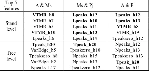
120 input features were ranked based on the scalar feature selection method to separate aspen and sugar maple, sugar maple and jack pine, aspen and jack pine, respectively. The top five features for each separation were listed in table 2, in which the features with bold font indicate they appeared at least twice in the three separation trials.
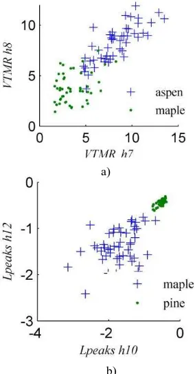
It is observed from table 2 that, at the stand level, most of the selected features belong to the VTMR andLpeaks feature groups. VTMR features seem good for separating aspen and sugar maple, which are both deciduous but the former one is intolerant and the latter one is tolerant species. Lpeaks features seem good for separating sugar maple and jack pine. To further investigate the importance of these two features groups, two scatter graphs
were plotted shown in figure 3a) and figure 3b). Figure 3a) shows the values of the features VTMR_h8 and VTMR_h7 derived from aspen and maple stands, and figure 3b) shows the values of the features Lpeaks_h12 and Lpeaks_h10 derived from maple and jack pine stands. It is shown in each scatter graph that there are very distinguish separations between the two species even though with some overlaps. Based on figure 3a), it is observed that aspen stands have higher VTMR values at 7th and 8th layers (some meters above the middle height 10th enough sunlight. Because of aspen’s shade tolerance property, these tree elements can not expend horizontally without enough sunlight to occupy as many gaps and space as maples. As a result, these leaves and branches are mostly concentrated around of tree truck, tending to be clumped pattern.
Top 5 selection method for each separation group for both of the stand and individual tree level. A: aspen;Ms: sugar maple;Pj: jack pine.
Based on figure 3b), it is observed that maple stands mostly have larger negative Lpeaks values at 11th and 12th layers (some meters below the middle height 10th layer of the stand) than jack pine stands. It indicates that the foliage of maple clumped more than jack pine at the two height layers. By visually examining the point clouds of the sample stands, this indication can be explained mostly by the following two reasons. The first reason is because the LiDAR points returned from the 11th and 12th height layers of maple stands are generally less than jack pine stands, and most of these returned LiDAR points are concentrated around tree trucks tending to be clumped pattern. The other reason is, even if as intolerant species, the jack pine stands have lots of spread dead branches in the two specific height layers, and these branches resulted in the returned LiDAR points to be dispersed. In addition, the jack pine stands also contain some shade tolerant understory plants growing up to the specific height layers. These understory plants will result in the returned LiDAR points to be more random and dispersed than maple stands.
In addition, the significance of selected features for individual tree level is not as obvious as for stand level. However, it is noticed that the Tpeak_h20 feature is significant as it was selected for all the three separations. This feature is derived from the lowest height layer of a tree containing mainly LiDAR points penetrated and returned from terrain and low vegetation, which is directly correlated with the gaps and clumping intensity of the upper canopy. For example, if the points returned from terrain are clumped, it probably means there are International Archives of the Photogrammetry, Remote Sensing and Spatial Information Sciences, Volume XXXVIII-5/W12, 2011
some gaps in the tree canopy so that the laser pulse is able to penetrate the canopy and hit the terrain.
Figure 3. Scatter graphs of VTMR and Lpeaks features for species separation at stand level.
4.2 Classification
The classification was tested based on different number of features selected by the two feature selection methods. Figure 4 shows how the overall classification changes with respect to the increasing number of features. The highest overall accuracy obtained at the stand level was 97.3% based on two features selected by PCA (figure 4b)), and at the tree level was 90% based on five features selected by PCA also. Generally, for all the classifiers, the overall accuracy not necessarily increases with the increasing number of features. The supervised classification methods are generally better than unsupervised methods according to the four graphs in figure 4. PCA has better performance and contribution than scalar feature selection method for the classification.
At the stand level, LDA was proved to be the most effective method with highest accuracy and relatively more robust than other classification methods (figure 4a) and 4b)). What’s more, it is noticed that the classification accuracy is very stable even the number of features changed, if PCA was used as the feature selection method (figure 4b)). In addition, EM classifier seems to be the worst classifier in this study due to the reason that we assume the features for each species only contain one Gaussian model, which may not correct for certain features and thus affect the performance of the EM classifier. At the individual tree level, DT was proved to be the most effective and robust method if features were selected by PCA (figure 4 d)). In addition, it is observed that by using just two features selected by scalar feature selection (i.e. Tpeaks_h20 and Npeaks_h12), the classification accuracy can be about 85% no matter which classifier was adopted (figure 4 c)).
a)
b)
c)
d)
Figure 4. Overall classification accuracy changes with the number of features selected by two feature selection methods, at a)
b)
the stand level (a) and b)) as well as the individual tree level (c) and d)).
5. CONCLUSIONS
This paper described the application of point pattern analysis in the classification of shade tolerant and intolerant species. The features newly derived from point pattern methods were proved effective for the species classification at the stand level and individual tree level. The linear discriminant analysis classifier was the best classifier for the classification at the both levels comparing with other three classifiers.
6. FUTURE WORKS
Besides to the number of features selected by feature selection methods and the choice of classifier, it is considered that there are some other factors may influence the feature values and thus influence the final classification accuracy. For example, the point density of LiDAR data, the quadrant size of Quadrant Count method, and the number of height layers for each object, etc. Therefore, more work should be done to analyze the sensitivity of these factors for the derivation of point patter features and the classification accuracy.
Species classification at individual tree level is more challenging than stand level due to the complex structure of trees. It is believed that some other features may also effective for the species separation at individual tree level such as echo types, intensity, and crown geometry, and thus the integration of these features will be investigated. Last but not least, some hierarchical methods will be proposed and exploited, considering the hierarchical relationships of types of species.
7. ACKNOWLEDGEMENTS
The authors would like to thank Natural Science and Engineering Research Council of Canada (NSERC), Canadian Space Agency (CSA), and GeoDigital International Inc.(GDI) for supporting the research, and also thank GDI for providing the high quality airborne LiDAR data for our research activity.
8. REFERENCE
Breiman, L., Friedman, J., Olshen, R., and Stone, C., 1984. Classification and Regression Trees. CRC Press, Boca Raton.
Craig, G. L., 1983. A test of the accuracy of shade-tolerance classifications based on physiognomic and reproductive traits. Canadian Journal of Botany, 61, pp. 1595-1598.
Dale, M. R. T., 1999. Spatial Pattern Analysis in Plant Ecology. Cambridge University Press, United Kingdom, pp. 1-6.
Diggle, P. J., 1983. Statistical Analysis of Spatial Point Patterns. Academic Press, London.
de Berg, M., Cheong, O., M. V., Kreveld, M. K., Overmars, 2008. Computational Geometry: Algorithms and Applications. Springer-Verlag, ISBN 978-3-540-77973-5.
Duda, R. O., Hart, P. E., and Stork, D. G., 2001. Pattern Classification. John Wiley & Sons, Inc., Canada.
Everitt, B. S., and Dunn, G., 2001. Applied Multivariate Data Analysis. Hodder Arnold, Great Britain, pp. 48-71.
Fortin, M-J., 2005. Spatial Analysis: A Guide for Ecologists. Cambridge University Press, New York, pp. 1.
Holmgren, J., Persson, Å., and Söderman, U., 2008. Species identification of individual trees by combining high resolution LiDAR data with multi-spectral images. International Journal of Remote Sensing, 29, pp. 1537-1552.
Pearson, K., 1901. On lines and planes of closest fit to systems of points in space. Philosophical Magazine, 2, pp. 559-572.
Reitberger, J., Krzystek, P., and Stilla, U., 2008. Analysis of full waveform LIDAR data for the classification of deciduous and coniferous trees. International Journal of Remote Sensing, 29(5), pp. 1407-1431.
Ripley, B. D., 1976. The second order analysis of stationary point processes. Journal of Applied Probability, 13, pp. 255-266.
Tariq, E., 2004. “Introduction to Point Pattern Analysis”. USA,
http://www.mcs.sdsmt.edu/rwjohnso/html/Point%20Pattern.doc
(accessed 25 April. 2011)
Theodoridis S., and Koutroumbas, K., 2006. Pattern Recognition, Academic Press, Elsevier, USA, pp. 224-233.
Vauhkonen, J., Tokola, T., Packalén, P., and Maltamo, M., 2009. Identification of Scandinavian Commerical Species of Individual Tree from Airborne laser Scanning Data Using Alpha Shape Metrics, Forest Science, 55(1), pp. 37-47.
Woods, M., Lim, K., and Treitz, P., 2008. Predicting forest stand variables from LiDAR data in the Great Lake - St. Lawrence Forest of Ontario. Forestry Chronicle, 84, pp. 827-839.