*Corresponding author. Tel.:#1 816 881 2761; fax:#1 816 881 2199. E-mail address:[email protected] (B.E. S+rensen).
The demand for risky assets: Sample selection
and household portfolios
William R.M. Perraudin
!
,
"
, Bent E. S
+
rensen
#
,
*
!Birkbeck College, London, UK"Bank of England, London, UK
#Federal Reserve Bank of Kansas City, Economic Research Department, 925 Grand Boulevard, Kansas City, MO 64198, USA
Received 1 May 1996; received in revised form 1 July 1999; accepted 1 October 1999
Abstract
We estimate a microeconomic model of household asset demands that allows for the fact that households typically have zero holdings of most assets. The adjustments for non-observed heterogeneity generalize methods developed by Dubin and McFadden (1984. Econometrica 52, 345}362). Simulating our model using a random sample of US households, we examine distributional and demographic e!ects on macroeconomic demands for money, stocks and bonds. ( 2000 Elsevier Science S.A. All rights reserved.
JEL classixcation: C35; E41; G11
Keywords: Discrete-continuous model; Consumer "nances; Monitoring costs; Incom-plete portfolios; Logit model
1. Introduction
This paper applies discrete-continuous econometric techniques to micro-economic data on household portfolio composition in order to estimate indi-vidual asset demands from the 1983 Survey of Consumer Finances (SCF). Since
1Flavin and Yamashita (1998) argue that housing wealth cannot be easily adjusted, but that the amount of housing wealth is likely to a!ect the choice between bond and stock holdings.
2Related papers which use household data to parameterize portfolio simulation models include Bertaut and Haliassos (1997) and Haliassos and Hassapis (1998).
3There is a large econometric literature on consumption demand with zero consumption of certain commodities. An early paper which uses censored regression models is Tobin (1958). See also Wales and Woodland (1983), Hanemann (1984), Lee and Pitt (1986) and Blundell and Meghir (1987).
the data set we study includes a random sample of the US population, by simulating our model, we obtain estimates of economy-wide money, stock and bond demand elasticities that fully allow for the non-linearities in asset demand generated by the combination of a discrete choice of asset portfolio with a continuous choice of quantities demanded for given portfolio composition.
Early research using cross-sectional, household-level data to investigate port-folio choices includes Uhler and Cragg (1971), Friend and Blume (1975) and King and Leape (1984). Recently, research in this"eld has become very active and several studies directly complement our own. Ioannides (1992) utilizes the panel data structure of the 1983 and 1986 SCFs, focusing particularly on changes in individual portfolios between these two dates. Hochguertel and van Soest (1996) examine how housing wealth a!ects total liquid"nancial wealth,1
and Poterba and Samwick (1997) use several waves of the SCF but focus exclusively on age versus cohort e!ects. Hochguertel et al. (1997) examine tax e!ects, Guiso et al. (1996) consider the relation between labor income risk and portfolio choice, and Heaton and Lucas (1997) study the e!ect of entrepreneurial risk on portfolio composition. Agell and Edin (1990) estimate a model resem-bling that of King and Leape on Swedish data, stressing tax e!ects in particular. Bertaut (1998) estimates bivariate probits on the 1983 and 1989 SCFs to investigate what determines whether households directly own stocks.2All the above studies, however, adopt reduced-form speci"cations and do not link discrete and continuous choices through utility maximization as is done in the present paper.
4The importance of non-marketed or illiquid assets for capital market equilibrium was stressed by Mayers (1972), Grossman and Laroque (1990) and Svensson and Werner (1993). Jones (1995) estimates the demand for home mortgage debt.
In the presence of"xed monitoring costs, one may decompose a household's optimal portfolio choice into (i) the choice of which assets to include in the portfolio and, (ii) the decision of how much of those assets to hold. The"rst stage involves comparing the maximum amount of utility attainable given di!erent incomplete portfolios, while the second stage may be viewed as a&continuous'
decision as to how much of each asset or liability to demand. Just as in standard consumer theory, Roy's identity implies demand functions for risky assets that are ratios of partial derivatives of the indirect utility function. Sandmo (1977) seems to have been the"rst to apply this technique in portfolio theory, but the present paper is the"rst to combine such an approach with discrete-continuous econometric methods.
The techniques applied in this paper, and in particular the selectivity adjust-ments, may be viewed as an extension of the methods developed for di!erent purposes by Dubin and McFadden (1984) (building on previous work by Heckman (1978)). Dubin and McFadden use discrete-continuous econometric methods to examine household consumption of di!erent forms of energy. While Dubin and McFadden only estimate a single demand function using limited information procedures, our study estimates the whole system simultaneously, imposing the cross-equation restrictions implied by the theoretical model. Extending Dubin and McFadden's selectivity adjustments to a multivariate system is non-trivial and may be regarded as one of the contributions of this paper.
The SCF provides detailed information on the asset holdings, income and demographic characteristics of a sample of 4262 US families. To estimate the model, we aggregate asset and liability holdings into stocks (S), bonds (B) and money (M). These categories are more highly aggregated than one might wish but including more assets is di$cult given the computational requirements of the estimation. Agents are all assumed to hold some quantity of money so investors may choose to hold any one of four di!erent sets of assets (SBM,SM,BM,M). Households in the SM category comprised less than 1% of the sample and were not included in the study since it would not be feasible to obtain estimates of the parameters relating to this regime with any precision.
5HARA utility functions are of the form:;(x)"(A#x)Bfor"xed parametersAandB. 6Stoker (1986) discusses the link between non-linearities and income distribution e!ects in aggregate equations. Lewbel (1996) and Jorgenson et al. (1982) examine the impact of aggregation e!ects in aggregate commodity demands.
Commonly adopted assumptions such as Hyperbolic Absolute Risk Aversion (HARA) preferences5or normally distributed rates of return imply individual and aggregate asset demands that are linear functions of initial wealth. To assess the importance of wealth distribution for aggregate portfolio demand, one may examine the extent to which individual demand functions are non-linear in wealth.6
We simulate our model for the actual dataset and for various perturbations to wealth distribution and demographics. The simulations allow for endogenous regime switching as households not only change their asset demands but also switch from holding one basket of assets to another. Our general"nding is that some forms of distributional shocks are very signi"cant. For example, redis-tributing wealth from poor to rich signi"cantly raises the demand for bonds. A proportionate rise in the wealth of all households, however, raises the demand for stocks. Some demographic changes are also important for aggregate asset demands. For example, a shift from married to single household heads raises the demand for bonds at the expense of that for stocks.
The paper is arranged as follows. Section 2 reviews our basic model of portfolio choice and describes its econometric implementation. Section 3 gives a brief account of the data used. Section 4 presents the results and reports on some tests of model speci"cation. Section 5 concludes.
2. The parametric model
2.1. Portfolio choice and Roy's identity
We begin by deriving the version of Roy's identity that forms the basis for our econometric model. Our approach follows that taken by Sandmo (1977) and Dalal (1983) in studying the comparative statics of risky asset demands. Suppose that an agent faces the following portfolio optimization decision:
max
Dn
G
E;
A
+N n/0D
n(1#rn)
B
such that +N n/0D
n"=
H
,whereD
n is the holding of assetn,rn is the rate of return on assetn, and=is
7The approach here described in a static setting may be generalized to a fully dynamic portfolio problem. In that case, the value functions described below become the maximized lifetime utility of an agent facing a multiperiod savings and portfolio problem. Since such value functions still depend on mean rates of return over the next period, the partial di!erential equations obtained below continue to hold.
8Parameterizing returns as we do is useful not because thehn parameters explicitly enter the econometric model but because it enables us to derive restrictions that must hold between demand and value functions.
9As noted in the Introduction, an alternative explanation of zero holdings is that agents face binding short-selling constraints as in Auerbach and King (1983). It appears unlikely, however, that the majority of households (and especially those with low wealth levels) have optimal, unconstrained portfolios which involve short selling stocks. It therefore seems to us worth exploring the alternative hypothesis that the large number of zero holdings re#ects costs of investing.
may parameterize the rates of return as: 1#r
0,h0, and 1#rn,hn#fn for
n"1,2,N, wherehn,E(1#rn) andfnis a random variable with zero mean.7
The"rst-order conditions to this problem are:
E[;@(=H
wherekis a Lagrange multiplier and=H
`1is the optimal, random future wealth.
For given returns, one may regard the "rst-order conditions as implicit func-tions ofkand the asset demandsD
n. Applying the implicit function theorem, one
may solve for the optimal demands,D
n, and substitute=H`1,+Dn(1#rn) into
where the last equality follows from the"rst-order condition for the safe asset. Combining equations in (2) gives
The relation in (3) is the counterpart to Roy's identity in deterministic consumer theory.
2.2. Modeling zero holdings
10These functions are not entirely arbitrary since the demand functions must satisfy Slutsky symmetry, additivity and homogeneity restrictions as in standard deterministic consumer theory.
11This amounts to assuming that part of the utility function is independent of wealth and mean asset returns. A monitoring cost is a simple interpretation of this term but it may also re#ect the fact that, for whatever reason, the household prefers to avoid certain portfolios.
costs, one may distinguish between (i) those (either "xed or proportional) incurred at the time when assets are bought or sold, and (ii) those (denoted
&monitoring costs') associated with holding particular asset combinations. Hali-assos and Bertaut (1995) discuss the latter type of costs and suggest they may explain why large numbers of households do not directly own stocks.
Theoretical studies of investors facing type (i) costs by Grossman and Laroque (1990), Dumas and Luciano (1991), and Davis and Norman (1990) show that such agents do not change their illiquid asset holdings if wealth changes by small amounts but adjust when wealth hits particular trigger levels. There is, however, no presumption with type (i) costs that zero holdings will be common. Type (ii) (monitoring-) costs appear a quite likely explanation of zero holdings. If they contain a"xed element, then such costs could also explain why low-wealth investors are particularly likely to have zero holdings of broad asset classes. For these reasons we explicitly model type (ii) costs in our empirical implementation below. Type (i) costs are implicitly included in that we analyze households' portfolio choices over liquid assets, conditioning on holdings of illiquid assets such as housing or mortgage debt for which transactions costs are large.
To derive our model, let<jidenote the value function of householdiwhen it
only invests in a subsetjof the total set of assets available. Here,j3sbm,bm,m
according to whether the household is in regimeSBM,BM, orM, respectively. One can then express the household's unconstrained value function,<
i, as <
i"maxM<sbmi ,<bmi ,<miN. (4)
The value function,< ji,<
ji(h,=
i,Xi), depends on household wealth,=i, and
a vector of variables describing the individual's demographic characteristics,X
i.
Suppose that<
jimay be written as
<ji"vji#eji,Hjx(h)X@
ibj#Hjw(h)(=i#wj0)1~o#X@iaj#eji (5)
forj"sbm,bm,m. Here,Hrx andHrw are functions of the mean asset returns,10
and the monitoring cost isX
iaj#eji.wj0 is a constant which equals minus the
12It may be seen as a drawback of the present approach that it is not more parsimonious in the parameterization it allows, but cross-sectional estimations of portfolio demands are typically conducted on large data sets (like the SCF used here), so parsimony is less of a concern.
13The indirect utility function in (5) may be taken to a power without changing the results, in which case (5) generalizes HARA by introducing a second power parameter,o. As Cass and Stiglitz (1970) show, HARA direct utility implies indirect utility functions that are themselves HARA in form. Whenois zero, it will turn out that demand functions are linear as they are for HARA preferences (see Cass and Stiglitz, 1970).
14If mutual fund separation holds, asset demands satisfy a rank restriction in that agents with di!erent initial wealths wish to hold di!erent combinations of a small number of mutual funds.
underlying utility function, we might expect to "nd restrictions across the parameters of the di!erent portfolios, but we do not impose such restrictions in the present study.12,13
The functional form in Eq. (5) is well-de"ned for positive wealth and repres-ents a monotonic transformation of the Price Independent Generalized Linear (PIGL) class of functional forms investigated by Muellbauer (1975) and (1976) in the context of consumer demand. The PIGL functional form in consumer theory may be written as<"FM(>1~o!a(p)1~o)/(b(p)1~o!a(p)1~o)Nwhere>is total
expenditure,pis a vector of prices,b(.) anda(.) are homogeneous and concave functions, andFis an arbitrary monotone function. The so-called Almost Ideal Demand System of Deaton and Muellbauer (1980) is a special case of this class of functions. For a survey of these and other functional forms commonly used in the context of consumer theory, see Blundell (1988).
Inverting the value function in (5) to obtain initial wealth as a function of utility and mean returns yields the agent's expenditure function, i.e., the min-imum cost of attaining a particular level of utility for given asset return distributions. Lewbel and Perraudin (1995) show that separability of the expen-diture function in prices is closely linked to mutual fund separation.14The PIGL form in (5) implies an expenditure function which is separable in functionals of the distribution of asset returns and, as we shall see below, yields mutual fund separation of order three.
For each conditional indirect utility function,<j, one may use Roy's identity,
as in Eq. (3), to derive conditional asset demand functions. Taking partial derivatives of Eq. (5) and substituting into Roy's identity yields
Djni"Djn(h,= i,Xi)
"h 0cjn#
h0LHjx/Lhn
(1!o)Hjw X@ibj(=i#wj0)o#
h0LHjx/Lhn
(1!o)Hjw(=i#wj0),
whereDjni is the demand for assetn(for n"0,2,Nj) of individuali holding
15Apart from possible di!erences in taxes.
16Since thebjparameters are identi"ed from the continuous demand part of the model, it would be simple to estimate the actualajparameters, but our interest is not focused on the parameter value per se.
17Basic references for such models are Maddala (1983) and McFadden (1984).
18McFadden (1973) shows that the assumption of iid Type I extreme valuedejis necessary and su$cient for the probabilities in the strict utility model to be logit, i.e., of the form
Pj"[exp(vj)]/[+kexp(vk)].
andbm) as
Dsbmsi "csbm
s #X@ibsbm(=i#wsbm0 )o#hsbmsw=i (6)
Dsbmbi "csbm
b #nbX@ibsbm(=i#wsbm0 )o#hsbmbw=i
Dbmbi"cbm
b #X@ibbm(=i#wbm0 )o#hbmbw=i. (7)
Since there is no price variation in our cross-sectional dataset,15we treathjnw as
"xed parameters to be estimated.
To implement the discrete choice model empirically, note"rst that an indi-vidual will select portfolio r if and only if: vr!vj*ej!er for all possible combinations of the available assets,j"sbm,bm,m. Thus, if we regard theej's as random variables distributed across the population, and normalize the
unidenti-"ed constantsHrx to one, it follows that
Pji,PrMhousehold with wealth=
i and characteristicsXi
chooses portfoliojN
"PrMvji!vki*eki!eji for all kOjN
"PrMX@
i(bj#aj!bk!ak)#Hj8(=i#wj0)1~o !Hk8(=
i#wk0)1~o* eji!ekifor all kOjN (8)
for allj"sbm,bm,m, where we treatHj8 and (aj#bj),j"sbm,bm,mas para-meters to be estimated.16
Eq. (8) is known as the strict utility model. We assume that the ej are iid, independent of wealth and demographic variables, and possess Type I extreme value distributions.17 In this case, the strict utility model is equivalent to a multinomial logit.18
19One may easily extend the argument to include a vector of unobserved demographics but this would make no di!erence to the estimation.
20The factor of proportionality is not identi"ed and is here normalized to unity. 21To identify the model, we setasbmu "!1 in the estimation.
2.3. Endogenous selection
Suppose that the vector of demographic variables takes the formX
i,(Zi,;i)
whereZ
iis a (K!1)-dimensional vector of observable demographic characteristics
and;
i is a scalar demographic variable not observable to the econometrician.19
Furthermore, decompose the parameter vector into sub-vectors corresponding to observed and unobserved demographic characteristics as aj"(aj0,aj6) and bj"
(bj0,bj6). The indirect utility function of a household in regimejmay be written as:
< ji"Z@
i(aj0#bj0)#Hj8(=i#wj0)1~o#uji, (9)
whereuji,(aj6#bj
6);i#eji, andejis de"ned as in the previous subsection. We
now adopt the following assumption:
Assumption. Suppose thatujfor j"1, 2,2,Jare independent, extreme-valued
random variables satisfying: E(;
iDusbmi , ubmi , umi)"+j/sbm,bm,mjjuji, where the
jjare constant parameters.
By an argument in Dubin and McFadden (1984), the expectation of the unobserved demographic conditional on the chosen portfolio of assets beingj, is proportional to20
E
jM;iN,EM;iDj"chosen portfolioN
"!jj logPji
(1!Pji)# +
k/sbm,bm,m
jkPkilogPki
(1!Pki), (10)
wherePjiis the logit probability that householdiholds portfolioj.
Now, adding the unobserved demographic term to the demand function derived in the previous subsection, we obtain portfolio-jspeci"c demand equa-tion
Djni"cjb#X@
ibj(=i#wj0)o#hjbw=i#;iaj6(=#wj0)o, (11)
which, with an obvious de"nition of the error term gives our"nal form
Djni"cjb#X@
ibj(=i#w0j)o#hjbw=ia6jEjM;iN(=#wj0)o#ljn. (12)
Djnis identical to the demand with no unobserved heterogeneity, except for the addition of a parameterized adjustment term,aj6E
jM;iN(=#wj0)o, plus an error
22We omit inconsequential constants.
(1984) refer to as the&Conditional Expectation Correction Method'. The adjust-ment terms in the demand equations introduce a large number of cross-equation restrictions between the discrete and continuous parts of the model.
2.4. Implementation
We assume that the error terms in the demand systems,l
n, are independently
distributed across households, but correlated across di!erent asset demands for a given household. Our speci"cation (see (11)) implies that error terms are heteroskedastic. Examination of the residuals from preliminary estimations indeed suggested pronounced heteroskedasticity, with the spread of the errors apparently proportional to liquid wealth,=. We, therefore, divided the
estima-tion equaestima-tions for the asset demands by (1#=) to achieve homoskedasticity.
We found that inclusion of a constant such as unity was necessary since, otherwise, households with liquid wealth close to zero received excessive weight and the algorithm failed to converge.
We de"ne l
sb"(lsbms , lsbmb ) and lb"(lbmb ), and assume that lsb is bivariate
normal with zero means and covariance matrixRSB whilel
b is an independent
normal random variable with a zero mean and scalar variance RB. Finally, de"ne 1
j forj"sbm, bm to be functions that equal unity if the household in
question holds the jth combination of assets.
The likelihood function for the complete model for each individual household is then:22
We estimate the total discrete-continuous model, including the& Dubin-McFad-den correction terms', simultaneously by substituting the parametric expres-sions for thevjand thel
k into Eq. (13).
23In this respect, our demand functions can be considered as&short-run' demand functions conditioned upon the&quasi-"xed'portfolios of property, etc. This approach parallels the notion of quasi-"xed inputs, such as the capital stock, in producer theory (see Nadiri, 1982).
24This was not particularly restrictive since liquid wealth includes just direct holdings of stocks, bonds and money and is much less than total net worth.
non-marketed assets.23 The illiquid asset holdings (including human capital, property value and mortgage debt) were introduced into the estimating equa-tions in the same way as the demographic variables.
The assumption implicit in this approach that holdings of non-traded or illiquid assets are exogenous as far as the estimation is concerned, is quite strong. The error terms in our model in part re#ect unobserved demographics which could possibly in#uence choices that investors have made in prior periods which result in their current holdings of house equity, mortgage debt, etc. If the in#uence were important, our approach would induce bias in our estimates, particularly of the non-traded asset parameters. Browning and Meghir (1991) estimate conditional commodity demand systems and comment on the assump-tions involved.
3. The data
We estimated the model using cross-sectional data drawn from the 1983 Federal Reserve Survey of Consumer Finances (SCF). The SCF includes both a random sample of 3,824 US families and a special additional sample of 438 high-income individuals selected from tax returns. The inclusion of this special high-income group makes the dataset well-suited for examining the demand for assets such as stocks which are held by only a small proportion of the popula-tion. Of the larger, random sample, we dropped 159 observations which had many missing variables. The sample contained some clear outliers. After experi-encing signi"cant convergence problems when these were included in the sample, we chose to restrict our analysis to households for which liquid wealth was less than one million dollars.24Our estimating sample (after leaving out the extremely small number of households that only held stocks and money) was 3353 observations.
The SCF contains much information about households'assets and liabilities as well as detailed data on demographic characteristics. The large number of zero holdings for di!erent asset types made it advisable to work with highly aggregated asset categories. We therefore supposed that individual investment decisions could be reduced at any one moment to the allocation of liquid wealth among stocks, bonds and money.
25An alternative might be to base portfolio selection on the liquidity services that households derive from asset holdings.
26The estimates are based on the model that includes selectivity adjustments in the demand functions. We also estimated a model without selectivity adjustments, obtaining broadly similar results.
our dual approach to portfolio decisions is consistent with a range of possible motives for holding di!erent portfolios.) We choose to think of the underlying utility function as depending on the total random monetary return (as described in Section 2).25Our focus is, therefore, on the riskiness of di!erent assets and we aggregate assets that we perceive as having similar risk characteristics. Stocks are taken to equal traded equities, bonds are de"ned as the sum of savings bonds, government securities and corporate bonds and money is represented by sight deposits plus savings accounts. Liquid wealth is the sum of money, bond, as stock holdings as we de"ne them.
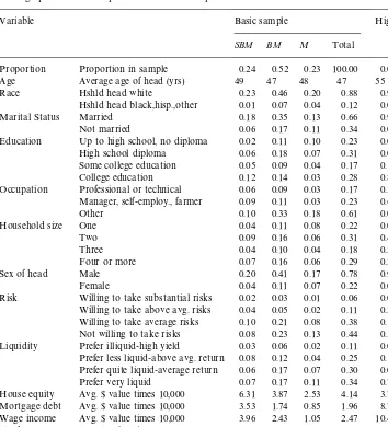
Table 1 shows the proportions of investors with di!erent demographic char-acteristics who held various possible combinations of assets. The table also gives the proportions of the basic random sample and of the high-income sample with particular characteristics. It is immediately apparent from the table that system-atic relationships exist between demographics characteristics and portfolio composition. For example, households which own stocks tend to have house-hold heads who are white, male, well-educated and in professional or adminis-trative employment. The attitudes of respondents to risk and liquidity also appear to be important, with households who report aversion to risk and a liking for liquid investments apparently less likely to hold stocks. Meanwhile, the high income sample, all but 11 of which hold all three assets, is overwhelm-ingly composed of households whose heads are white, educated, married with a marked preference for risky, illiquid, high return investments.
4. Results
4.1. Value function parameters
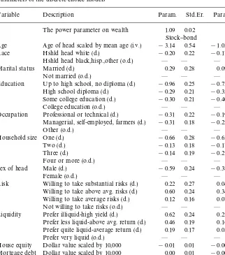
Table 2 presents estimates from the discrete choice part of the model.26
A crucial parameter is the non-linearity parameter,o. This appears in the"rst row of Table 2 and is estimated to be 1.09. The estimate di!ers in a statistically signi"cant way from the value of unity which would imply linear demand functions. We investigate the economic signi"cance of this degree of non-linearity below. The parameters, wj0, that capture the minimum allowable
Table 1
Demographic factors and portfolio choice. Descriptive statistics!
Variable Basic sample High income
SBM BM M Total
Proportion Proportion in sample 0.24 0.52 0.23 100.00 0.02
Age Average age of head (yrs) 49 47 48 47 55
Race Hshld head white 0.23 0.46 0.20 0.88 0.99
Hshld head black,hisp.,other 0.01 0.07 0.04 0.12 0.01
Marital Status Married 0.18 0.35 0.13 0.66 0.91
Not married 0.06 0.17 0.11 0.34 0.09
Education Up to high school, no diploma 0.02 0.11 0.10 0.23 0.01
High school diploma 0.06 0.18 0.07 0.31 0.03
Some college education 0.05 0.09 0.04 0.17 0.12
College education 0.12 0.14 0.03 0.28 0.84
Occupation Professional or technical 0.06 0.09 0.03 0.17 0.30 Manager, self-employ., farmer 0.09 0.11 0.03 0.23 0.66
Other 0.10 0.33 0.18 0.61 0.04
Household size One 0.04 0.11 0.08 0.22 0.07
Two 0.09 0.16 0.06 0.31 0.44
Three 0.04 0.10 0.04 0.18 0.20
Four or more 0.07 0.16 0.06 0.29 0.29
Sex of head Male 0.20 0.41 0.17 0.78 0.97
Female 0.04 0.11 0.07 0.22 0.03
Risk Willing to take substantial risks 0.02 0.03 0.01 0.06 0.09 Willing to take above avg. risks 0.04 0.05 0.02 0.11 0.21 Willing to take average risks 0.10 0.21 0.08 0.38 0.19 Not willing to take risks 0.08 0.23 0.13 0.44 0.51 Liquidity Prefer illiquid-high yield 0.03 0.06 0.02 0.11 0.07 Prefer less liquid-above avg. return 0.08 0.12 0.04 0.25 0.10 Prefer quite liquid-average return 0.06 0.17 0.07 0.30 0.05
Prefer very liquid 0.07 0.17 0.11 0.34 0.79
House equity Avg.$value times 10,000 6.31 3.87 2.53 4.14 3.74 Mortgage debt Avg.$value times 10,000 3.53 1.74 0.85 1.96 8.77 Wage income Avg.$value times 10,000 3.96 2.43 1.05 2.47 10.49
Stocks Avg.$value times 10,000 5.51 0.00 0.00 1.32 10.55
Bonds Avg.$value times 10,000 4.39 1.65 0.00 1.91 13.22
Money Avg.$value times 10,000 2.53 0.96 0.41 1.21 8.19
Liquid assets Avg.$value times 10,000 12.43 2.61 0.41 4.44 31.96
Table 2
Parameters of the discrete choice models
Variable Description Param. Std.Er. Param. Std.Er.
o The power parameter on wealth 1.09 0.02
Stock}bond Bond
Age Age of head scaled by mean age (i.v.) !3.14 0.54 !1.03 0.36
Race Hshld head white (d.) !0.20 0.22 !0.17 0.14
Hshld head black,hisp.,other (o.d.) * * * *
Marital status Married (d.) 0.29 0.28 0.09 0.19
Not married (o.d.) * * * *
Education Up to high school, no diploma (d.) !0.96 0.25 !0.73 0.17
High school diploma (d.) !0.29 0.21 !0.32 0.16
Some college education (d.) !0.30 0.21 !0.40 0.16
College education (o.d.) * * * *
Occupation Professional or technical (d.) !0.31 0.22 !0.19 0.16 Managerial, self-employed, farmers (d.) !0.31 0.18 !0.22 0.13
Other (o.d.) * * * *
Household size One (d.) !0.66 0.28 !0.65 0.19
Two (d.) !0.13 0.18 !0.17 0.13
Three (d.) !0.14 0.19 !0.21 0.14
Four or more (o.d.) * * * *
Sex of head Male (d.) !0.59 0.24 !0.38 0.16
Female (o.d.) * * * *
Risk Willing to take substantial risks (d.) 0.22 0.27 0.04 0.20 Willing to take above avg. risks (d.) 0.60 0.24 0.34 0.19 Willing to take average risks (d.) 0.12 0.16 0.07 0.11
Not willing to take risks (o.d.) * * * *
Liquidity Prefer illiquid-high yield (d.) 0.62 0.24 0.23 0.18 Prefer less liquid-above avg. return (d.) 0.46 0.19 0.16 0.14 Prefer quite liquid-average return (d.) 0.19 0.17 0.05 0.12
Prefer very liquid (o.d.) * * * *
House equity Dollar value scaled by 10,000 !0.01 0.01 !0.00 0.01 Mortgage debt Dollar value scaled by 10,000 0.00 0.01 !0.00 0.01 Wage income Dollar value scaled by 10,000 0.13 0.04 0.14 0.04
Constant Constant term 17.37 3.67 8.69 1.68
Wealth Slope term on=1~o !14.48 3.64 !5.69 1.62
27The coe$cients which appear in the table, e.g., for the stock}bond}money regime, represent
asbm#bsbm!(am#bm) in the notation of the theoretical model, except for the parameter in the bottom row which equalsHsbm8 !Hm8.
28These categories were consolidated based on initial exploratory estimations, which showed similar coe$cients for, e.g., heads in professional and technical occupations.
appears to play a role since high school drop-outs are less likely and college graduates more likely to hold both stocks and bonds. Age appears strongly signi"cant in that families with older heads seem to be less likely to have non-zero bond holdings and even less likely to have non-zero equity holdings. This result should be interpreted with caution, since age e!ects cannot be separated from cohort e!ects in a single cross-section. Poterba and Samwick (1997) document signi"cant cohort e!ects using several waves of the SCF.
Of the variables which describe households'attitudes to di!erent investments, those re#ecting attitudes to liquidity a!ect portfolio composition in an intuitive fashion. Households which prefer illiquid high-yield investments are signi" -cantly more likely to hold stocks, while those which prefer less liquid invest-ments are also more likely to hold stocks although to a lesser degree. The variables measuring attitudes towards risk yield less intuitive results. The estimates suggest that households which expressed willingness to&take substan-tial"nancial risks'are not signi"cantly di!erent from individuals who claim to be¬ willing to take any"nancial risks'. On the other hand, individuals who
&take above average"nancial risks', are signi"cantly more likely to holds stocks. Variables which do not have a signi"cant e!ect on portfolio composition include race, marital status and occupation, although in the case of occupation there is some evidence that households with heads in professional, technical, or managerial occupations or who are self-employed28 are less likely to hold stocks. The fact that these variables have little impact may appear surprising, but one should recall that this is a marginal e!ect, holding education and risk-and liquidity-attitudes constant.
Of the continuous variables, wage income signi"cantly in#uences portfolio composition in that households with higher income are more likely to hold bonds or stocks. Total liquid wealth also has a very strong in#uence on the probabilities of holding bonds and stocks. We do not"nd that holdings of house equity or mortgage debt a!ect portfolio composition.
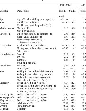
4.2. Parameters of the conditional demand functions
Table 3
Parameters from the continuous demand systems
Stock}bond Bond
Variable Description Param. Std.Er. Param. Std.Er.
Stock
Age Age of head scaled by mean age (i.v.) !45.89 11.13 11.01 9.60
Race Hshld head white (d.) !2.33 3.43 0.09 3.20
Hshld head black,hisp.,other (o.d.) * * * *
Marital status Married (d.) 1.15 3.16 !0.97 3.68
Not married (o.d.) * * * *
Education Up to high school, no diploma (d.) !3.79 2.80 !0.12 3.33
High school diploma (d.) 0.57 2.03 4.16 2.14
Some college education (d.) 0.68 1.84 1.85 2.19
College education (o.d.) * * * *
Occupation Professional or technical (d.) !3.93 1.92 !0.83 2.27 Managerial, self-employed, farmers (d.) !2.03 1.63 !5.49 1.94
Other (o.d.) * * * *
Household size One (d.) 2.10 3.52 !8.71 3.97
Two (d.) 2.52 1.67 0.05 1.99
Three (d.) 0.41 1.87 !4.43 2.19
Four or more (o.d.) * * * *
Sex of head Male (d.) 1.49 2.79 !8.21 3.05
Female (o.d.) * * * *
Risk Willing to take substantial risks (d.) 0.68 2.36 2.37 2.89 Willing to take above avg. risks (d.) 1.45 1.84 !0.96 2.72 Willing to take average risks (d.) !2.29 1.86 !0.02 1.71
Not willing to take risks (o.d.) * * * *
Liquidity Prefer illiquid-high yield (d.) !1.64 2.24 6.32 2.64 Prefer less liquid-above avg. return (d.) 0.13 2.03 !1.76 2.29 Prefer quite liquid-average return (d.) !2.09 2.10 0.87 2.03
Prefer very liquid (o.d.) * * * *
House equity Dollar value scaled by 10,000 0.01 0.04 !0.03 0.05 Mortgage debt Dollar value scaled by 10,000 0.02 0.08 !0.15 0.11 Wage income Dollar value scaled by 10,000 !0.13 0.08 0.13 0.09
Constant (Multiplies=o) 53.98 17.93 19.01 36.18
Wealth Slope term on= 16.54 18.16 16.70 34.95
Constant Constant !0.59 3.21 0.00 0.92
Bond
Constant Proportionality termnb !1.63 0.44
Wealth Slope term on= 108.20 34.86
29The parameters are not identi"ed non-parametrically and it is therefore possible that the parameter estimates re#ect other mis-speci"cation of the model.
30Recall that the coe$cientbsbm6 which measures the impact of the unobserved heterogeneity on stock demand is normalized to}1.
Table 4
Selectivity adjustment parameters
Parameter t-Stat.
jsbm !15.67 7.24
jbm 6.06 6.49
jm !47.07 24.37
abmu !1.21 0.70
The estimates suggest that asset demands are signi"cantly in#uenced by age in that older households hold less stocks and more bonds. As noted above, this age e!ect may in fact re#ect changes between cohorts. Occupation also has a signi"cant impact. Households whose heads are in professional or technical occupations demand signi"cantly less stocks, while managers and self-employed demand signi"cantly less bonds in the bond regime. Attitudes towards risk and liquidity do not seem to have strong e!ects on the demand for risky assets in the stock}bond}money regime. In the bond regime, on the other hand, we observe a large and signi"cant estimate of bond demand for individuals who prefer illiquid high-yield assets. Holdings of housing equity and mortgage debt do not have a signi"cant impact on asset demands.
A high level of wage income may imply higher bond holdings in both the stock}bond}money regime and the bond}money regime, but in neither regime is the coe$cient signi"cant at the 5% level. Not surprisingly, the amount of liquid wealth has a strong impact on asset holdings. Since wealth changes in the model have non-linear e!ects which vary across demographic groups, they are best illustrated by simulations which we report below.
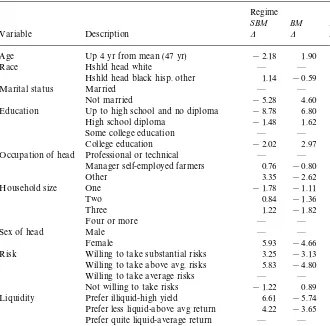
4.3. Selectivity adjustment
Table 5
Demographic factors and portfolio regime!
Regime
SBM BM M
Variable Description D D D
Age Up 4 yr from mean (47 yr) !2.18 1.90 0.28
Race Hshld head white * * *
Hshld head black hisp. other 1.14 !0.59 !0.55
Marital status Married * * *
Not married !5.28 4.60 0.67
Education Up to high school and no diploma !8.78 6.80 1.98
High school diploma !1.48 1.62 !0.14
Some college education * * *
College education !2.02 2.97 !0.96
Occupation of head Professional or technical * * *
Manager self-employed farmers 0.76 !0.80 0.04
Other 3.35 !2.62 !0.74
Household size One !1.78 !1.11 2.89
Two 0.84 !1.36 0.52
Three 1.22 !1.82 0.60
Four or more * * *
Sex of head Male * * *
Female 5.93 !4.66 !1.28
Risk Willing to take substantial risks 3.25 !3.13 !0.12
Willing to take above avg. risks 5.83 !4.80 !1.04
Willing to take average risks * * *
Not willing to take risks !1.22 0.89 0.33
Liquidity Prefer illiquid-high yield 6.61 !5.74 !0.88
Prefer less liquid-above avg return 4.22 !3.65 !0.57
Prefer quite liquid-average return * * *
Prefer very liquid !3.61 3.18 0.43
House owner Zero house equity and mortgage 0.04 0.04 !0.08
Wage income Double sample average !0.13 1.08 !0.95
!Note: Entries represent changes in regime probabilities multiplied by 100. Dashes indicate baseline categories. The baseline household has four or more members and has a white married household head with some college education, a professional occupation, is willing to take average risks, requires average liquidity holds house equity and mortgage debt equal to the sample averages and is of average age.
4.4. Simulations
Demographic factors and asset demands!
Discrete-contin. model Reduced-form model
SBM BM SBM BM
Stock Bond Bond Stock Bond Bond
Variable Description D D D D D D
Age Up 4 yr from mean (47yr) !9.31 15.19 2.24 !12.04 12.04 2.31
Race Hshld head white * * * * * *
Hshld head black hisp. other 11.81 !19.26 !0.44 25.53 !24.65 !2.73
Marital status Married * * * * * *
Not married !5.85 9.54 4.94 !10.57 2.99 5.57 Education Up to high school and no diploma !22.67 36.98 !9.99 1.75 29.76 2.89 High school diploma !0.55 0.90 11.73 7.74 !4.95 10.31
Some college education * * * * * *
College education !3.44 5.61 !9.40 !16.71 !10.21 !18.88 Occupation of head Professional or technical * * * * * *
Manager, self-employed, farmers 9.65 !15.74 !23.62 !0.98 !13.25 !22.33 Other 19.93 !32.50 4.23 9.39 !29.71 2.78 Household size One 10.64 !17.35 !44.17 34.19 !4.07 !27.33 Two 12.79 !20.87 0.26 19.44 !14.34 5.88 Three 2.07 !3.37 !22.48 12.74 1.50 !17.48
Four or more * * * * * *
Sex of head Male * * * * * *
Female !7.58 12.37 41.67 !12.94 18.36 38.32 Risk Willing to take substantial risks 15.05 !24.55 12.12 24.96 !15.01 16.04 Willing to take above avg. risks 18.96 !30.92 !4.73 15.99 !21.87 !5.72 Willing to take average risks * * * * * * Not willing to take risks 11.61 !18.94 0.12 26.25 !22.13 1.03 Liquidity Prefer illiquid-high yield 2.30 !3.75 27.64 8.61 4.23 26.20 Prefer less liquid-above avg return 11.30 !18.43 !13.35 1.96 !9.80 !14.80 Prefer quite liquid-average return * * * * * * Prefer very liquid 10.63 !17.33 !4.43 8.82 !25.22 !4.59 House owner Zero house equity and mortgage !0.31 0.51 2.06 !0.93 0.35 1.34 Wage income Double sample average !1.62 2.65 1.60 !2.42 !0.25 0.25
!Note: Entries represent changes and percentage changes in asset demands expressed in units of$100. Dashes indicate baseline categories. The baseline household has four or more members and has a white married household head with some college education a professional occupation is willing to take average risks and requires average liquidity who holds household equity and mortgage debt equal to the sample averages and is of average age.
The baseline household contains four or more members, has a white, married household head with some college and a professional occupation, and is willing to take average risk while requiring average liquidity. House equity, mortgage debt, the wage income and age of the household head are set equal to the sample averages.
The economically most important e!ects on the probability of being in di!erent regimes are age, marital status, education, sex of household head and risk and liquidity attitudes. If a household head is four years older, the likeli-hood of being in theSBMregime falls by 2.18%, with corresponding increases in
BM and M probabilities of 1.90% and 0.28%. An unmarried household is a substantial 5.28% less likely to be in theSBMregime and 4.60% more likely to be in theBMregime. Female household heads are 5.93% more likely to be in the
SBMregime, with theBMandMregime probabilities being 4.66% and 1.28% lower.
Those with some college education are the most likely to be in the SBM
regime. Households whose heads have no high school diploma are between about 9% less likely to be in theSBMregime. Such households are 7% more likely to hold BM portfolios and 2% more likely to hold just money. Risk attitudes signi"cantly a!ect regime probabilities in that those willing to take above average risks or greater are 3% to 6% more likely to be in the SBM
regime than those unwilling to take any risks. Liquidity attitudes are even more important in that households preferring illiquid or less liquid investments with higher returns are 4% to 7% more likely to hold all three asset categories than households which favor very liquid investments.
Table 6 reports the impact on conditional asset demands of changes in the characteristics of the reference household described above. Changes in demand are expressed in units of$100. The left hand three columns give the changes in demands forecast by the discrete-continuous model while columns 4}6 show the changes implied by reduced form asset demands (explained more fully below). The results based on our own discrete-continuous model suggest that a large number of factors can substantially a!ect asset demands conditional on being in one or other regime. Some variables such as race, occupation and household size which did not in#uence regime probabilities in an economically signi"cant way do greatly a!ect continuous demands. In particular, those not in professional or managerial occupations are likely to hold $2000 more stocks and$3200 less bonds in theSBMregime. Households with only one member hold$1700 less in bonds in the SBM regime and a surprisingly $4200 less in bonds in the BM
regime.
Risk attitudes are important in that households which are willing to take above average risks or greater hold$1500 to$1900 more in stocks and$2500 to
31We estimated these regressions by maximizing the part of the likelihood for the demand equations without imposing cross equation restrictions between the di!erent demand functions in theSBMregime. We setoto 1.09 (the value we obtained in our estimation of the full model) rather than estimating it freely and omitted the selectivity terms.
Columns 4}6 of Table 6 report simulations based on reduced form regressions in which the demand functions are estimated alone.31This permits us to see to what extent our simulations are in#uenced by the cross-equation constraints introduced by the selectivity adjustment and the restriction across parameters in the demand functions of theSBMregime. The signs and broad magnitudes of the e!ects in columns 4}6 of the table match up to a considerable degree with those in columns 1}3. As one might imagine, the e!ects which appear the most similar between the reduced form models and the discrete-continuous are those like age which are associated with parameters bearing low standard errors.
It is interesting to note that the e!ects of risk and liquidity attitudes appear even more&non-monotonic'in the reduced form model. For example, categories of household which express preferences for high risk}high return investments and those which prefer to take no risks are both likely to hold more stocks than households willing to take average risks and the magnitudes of the e!ects are greater than in the discrete-continuous model.
4.5. Macroeconomic simulations
Since the SCF contains a randomly selected sample of the US population (for information on how the sample was constructed, see Avery and Elliehausen (1986)), we were able to simulate our model in such a way as to mimic the macroeconomic e!ects of changes in the demographic or wealth pro"le of the population as a whole. To do this, we calculated the aggregate asset demands by (i) for each household in the random sample, calculating the "tted regime-speci"c demands weighted by the "tted regime probabilities, (ii) sum these weighted household-level demands across the entire random sample. Having accomplished this for the random sample, we altered demographic or other characteristics of the random sample, recalculated the aggregate asset demands and then worked out the per capital change (measured in units of$100) in the aggregate demands.
The results of these calculations are contained in Table 7. The"rst four rows in the table show the percentage impacts on aggregate demands and fractions of the portfolio holding di!erent asset combinations of changes in the population liquid wealth pro"le. A 10% proportionate rise in each household's liquid wealth leads to a 1.3% increase in the fraction of the population in theSBM
Macroeconomic simulations!
Changes in
No. Simulation Stock demand Bond demand Money demand SBM BM M Prob. Prob. Prob.
1. 10% proportional rise in wealth 3.50 4.72 !48.22 1.31 !0.51 !0.81 2. Lump sum rise in wealth 7.92 20.74 !28.66 1.97 14.14 !16.10 3. Increase log wealth dispersion 10.60 2.39 !12.98 !4.06 !9.33 13.39 4. Switch wealth from poor to rich 4.22 14.41 !18.63 0.69 15.21 !15.90 5. Increase age by 10% !18.03 21.83 !3.80 !1.85 1.22 0.63 6. Increase age by 5% of mean age !7.20 11.42 !4.21 !0.72 0.42 0.30 7. Raise educational level 1 category 1.33 3.47 !4.80 0.42 2.24 !2.65 8. 40% of households shrink in size 1.00 0.46 !1.46 0.06 !0.72 0.66 9. 40% hshlds. shift up occupation !5.68 11.10 !5.42 !0.27 !0.30 0.57 10. 40% hshlds. shift married to single !7.51 7.54 !0.03 !1.76 1.67 0.09 11. 40% hshlds. shift male to female !2.13 16.12 !13.99 1.76 !1.43 !0.33 12. Fall in risk aversion by 1 category !4.44 12.82 !8.38 0.36 0.30 !0.66 13. Fall in liquidity pref. by 1 category !4.56 14.44 !9.88 0.54 !0.18 !0.36 14. 20% rise in house equity and mortgage !0.05 2.89 !2.83 !0.09 0.06 0.03 15. 20% rise in wage !0.05 2.89 !2.83 !0.09 0.06 0.03 16. Raise educational level 1 category !12.77 27.81 !15.04 !0.03 2.95 !2.92 17. 40% hshlds. shift married to single !4.03 !20.42 24.45 !5.85 5.13 0.72
!Note: entries are per capita changes in demands in units of$100 and changes in regime probabilities in percent. Changes in demands are&total'in that they include the e!ects of regime switches by individual households. Notes on Simulations: 1. All wealths rise 10%. 2. All wealths rise by 10% of mean wealth. 3. The absolute deviation of log wealth from mean log wealth is increased by 10%. 4. 10% of wealth of those with wealth less than the mean is redistributed in equal lump sum amounts to those with wealth grater than the mean. 5. Ages of household heads rise by 10% of amount they exceed 16 y. 6. Ages of household head increase by 5% of mean age. 7. Educational categories increase by 1. 8. 40% of households shrink in size by 1 category. 9. 40% of households shift to higher status profession by 1 category. 10. 40% of household heads if male shift to female. 11. 40% of household heads if married shift to single. 12. Risk aversion falls by 1 category. 13. Illiquidity aversion falls by 1 category. 14. House equity and mortgage debt rises by 10%. 15. Wage rise by 10%. 16. Like 7 except risk and liquidity attitudes and occupations generated endogenously. 17. Like 10 except risk and liquidity attitudes and occupations generated endogenously.
W.R.M.
Perraudin,
B.E.
S
~
rensen
/
Journal
of
Econometrics
97
(2000)
117
}
32&Professional and technical' is regarded as the highest and &Other' as the lowest status profession.
just money and 0.5% from households which own bonds and money. Interest-ingly, the e!ect of the regime switches by households and the intra-regime substitutions lead to roughly equal increases in stocks and bonds at the expense of aggregate money holdings.
A lump-sum (rather than proportionate) increase in liquid wealth for all households in the population leads to substitution from money to bonds much more than to stocks, as one may see from the second row of Table 7. This suggests that to obtain large increases in stock demand, liquid wealth growth must be concentrated on the rich. This impression is con"rmed by the two simulations we perform for increases in liquid wealth inequality (rows 3 and 4 of the table). Raising the dispersion of log wealth (which signi"cantly raises the wealth of the very rich) boosts stock demand substantially whereas just switch-ing wealth from those below to those above the mean wealth leads to more marked increases in aggregate bond demand.
Rows 5 to 15 of Table 7 contain simulations of shifts in population demo-graphics. Age has a major impact (although as already noted, this is probably in large part a cohort e!ect). Raising educational levels has surprisingly little impact on aggregate asset demands although it does lead quite a few households to switch from theMto theBMregime. Changes in profession have a large impact on asset demands with shifts towards higher profession status32leading to a fall in stock demand and an increase in bond demand. In this case, most of the e!ect is intra-regime in that the fractions of the population holding di!erent asset combi-nations are little changed. By contrast, the substitutions from stocks to bonds that occurs when more households have single and female rather than married and male household heads seems to operate mostly through regime switches. Lastly, rows 14 and 15 of Table 7 show that falls in risk aversion or liquidity preference, although they induce households to switch into theSBMregime, increase bond rather than stock demand, largely at the expense of demand for money.
and marital status on aggregate asset demand by (i) altering the &exogenous'
educational status and marital status dummies as they appear directly in the regime probabilities and the demand functions, and (ii) changing the forecast values of the&endogenous'dummies by changing the&exogenous'dummies in the logit forecasting model.
The results underline how e!ects may be altered by looking at&total'rather than &marginal' e!ects of demographic shifts. A rise in educational level now actually leads to a fall in stock demand because it generates not just a positive direct e!ect on stock demand but also negative indirect e!ects by pushing households into more professional occupational status and leading them to have less risk averse and less illiquidity averse attitudes. These latter indirect e!ects boost bond demand as we have already seen. The impact of a shift from married to single household head is again signi"cantly di!erent if one looks at the total rather than the marginal e!ect. In the total e!ect simulation, bond demand falls signi"cantly rather than rising.
4.6. Specixcation tests
We spent some considerable time investigating the speci"cation of the model. Thus, we examined if the parameters were multicolinear through a series of estimations where we varied the set of included demographic variables. We found that the variables in the tables above, seemed not to display excessive variation when other demographic variables were left out. In a previous version, we included a squared term in age, but we found the coe$cient to this term to be highly correlated with other variables leading to estimates which were sensitive to speci"cation. We therefore left out this term (with some regret since a non-linearity term in age appears desirable).
We experimented with di!erent forms of heteroskedasticity correction. This proved to be quite a sink for CPU time, since with more complicated forms (especially if a parameter was included in the heteroskedasticity term), it was extremely di$cult to obtain convergence. We therefore decided to adopt the simple form 1#=. With this adjustment, the"tted residuals from the demand equations
showed no obvious dependence on wealth when plotted and we concluded that further attempts to reduce heteroskedasticity were probably not worthwhile.
To check our distributional assumption, we calculated the skewness and kurtosis coe$cients of the three sets of demand function residuals (the stock and bond demands from the SBM regime and the bond demand from the BM
Finally, we split the sample into those with wealth less than and greater than the median level and performed a Chow test to see if the estimated coe$cients di!ered across high and low wealth samples. The model clearly #unked this test. The estimates were, however, not very well determined on the sub-samples and we did not attempt to construct a larger more complicated model with further non-linea-rity to pass this hurdle. (Recall that all other work in this area, to our knowledge, estimates reduced formlineardemand functions.) Rather we suggest further explo-ration of models of portfolio demand utilizing parsimonious parametric functions, consistent with utility optimization, as an open area for further research.
5. Conclusion
This paper has employed discrete-continuous econometric methods, allowing for sample selectivity, to model US households'portfolio decisions. Our major conclusions are:
1. Asset Engel curves are non-linear, generating signi"cant increases in de-mands for stocks and bonds as wealth rises. In a simulation designed to replicate the impact on the portfolio choices of the US population, we"nd that a 10% proportional rise in wealth of all households leads to a 24% and a 25% increase in stock and bond demand, respectively. A 10% rise in the absolute dispersion of log wealth leads to a 11% rise in stock demand but only a 2% rise in the demand for bonds.
2. Household characteristics apart from wealth have important e!ects on port-folio decisions. For individual households, family size, sex of household head, education and attitudes to risk and liquidity signi"cantly in#uence the basket of assets households end up possessing. Race, marital status, and occupation are less important.
3. Simulations of the impact of changes in household characteristics on the asset demands of the population as a whole suggest that shifts from married to single household heads, changes in educational level, occupation, liquidity and risk preference can lead to big percentage changes in bond demands, often with o!setting changes in both stock and money demands.
4. Selectivity adjustments are highly statistically signi"cant. This suggests that the results of past studies which employed discrete-continuous methods but did not allow for selectivity may be hard to interpret.
Acknowledgements
herein are solely those of the authors and do not necessarily re#ect the views of the Bank of England, the Federal Reserve Bank of Kansas City or the Federal Reserve System.
Appendix A. Data:The survey questions
1. Age of head: Question: age by date of birth, at last birthday of head of household. All missing values imputed. (Range: 16}60).
2. Race of household: Variable is observed race of survey respondent. All missing values imputed using census data and other sources. Categories: (i) Caucasian except hispanic; (ii) black except hispanic; (iii) hispanic; (iv) American indian or Alaskan native; (v) Asian or paci"c islander; (vi) NA. 3. Marital status: Question: marital status. Responses: (i) married (includes
couples living together); (ii) separated; (iii) divorced; (iv) widowed; (v) never married; (v) married but spouse not present.
4. Education of household head: Question: education of household head. Re-sponses: (i) 0}8 grades; (ii) 9}12 grades, no high school diploma; (iii) high school diploma or equivalent, no college; (iv) some college, no college degree; (v) college degree.
5. Occupation of head: Question: occupation of household head. Response: (i) professional, technical and kindred workers; (ii) managers and adminis-trators (except farm); (iii) self-employed managers; (iv) sales, clerical and kindred workers; (v) craftsmen, protective service, and kindred workers; (vi) operatives, laborers, and service workers; (vii) farmers and farm managers; (viii) miscellaneous (mbrs. of armed service, housewives, students, never worked and other occupations).
6. Household size: Question: total number of persons in household. Responses: (i) 1; (ii) 2; (iii) 3; (iv) 4; (v) 5; (vi) 6; (vii) 7; (viii) 8; (ix) 9; (x) 11; (xi) 13. 7. Sex of household head: Question: sex of head of household. Responses: (i)
male; (ii) female.
10. Value of home: Current value of home.
11. House mortgage: Sum of"rst and second mortgages on household's primary residence.
References
Agell, J., Edin, P.-A., 1990. Marginal taxes and the asset portfolios of Swedish households. Scandina-vian Journal of Economics 92, 47}64.
Auerbach, A.J., King, M.A., 1983. Taxation, portfolio choice and debt-equity ratios: a general equilibrium model. Quarterly Journal of Economics 98, 587}609.
Avery, R.B., Elliehausen, G.E., 1986. 1983 Survey of consumer"nances, Avery/Elliehausen cleaned sample tape manual. Board of Governors of the Federal Reserve System mimeo.
Bertaut, C.C., 1998. Stockholding behavior of U.S. households: evidence from the 1983-1989 Survey of Consumer Finances. Review of Economics and Statistics 80, 263}275.
Bertaut, C.C., Haliassos, M., 1997. Precautionary portfolio behavior from a life-cycle perspective. Journal of Economic Dynamics and Control 21, 1511}1542.
Blundell, R., 1988. Consumer behavior: theory and empirical evidence * a survey. Economic Journal 98, 16}65.
Blundell, R., Meghir, C., 1987. Bivariate alternatives to the Tobit model. Journal of Econometrics 34, 179}200.
Browning, M., Meghir, C., 1991. The e!ect of male and female labor supply on commodity demands. Econometrica 59, 925}951.
Cass, D., Stiglitz, J.E., 1970. The structure of investor preferences and asset returns and separability in portfolio allocation: a contribution to the pure theory of mutual funds. Journal of Economic Theory 2, 122}160.
D'Agostino, R.B., Belanger, A., D'Agostino Jr., R.B., 1990. A suggestion for using powerful and informative tests of normality. American Statistician 44, 316}321.
Dalal, A.J., 1983. Comparative statics and asset substitutability-complementarity in a portfolio Model: a dual approach. Review of Economic Studies 50, 355}367.
Davis, M.H.A., Norman, A.R., 1990. Portfolio selection with transactions costs. Mathematics of Operations Research 15, 676}713.
Deaton, A.S., Muellbauer, J., 1980. An almost ideal demand system. American Economic Review 70, 312}326.
Dubin, J.A., McFadden, D.L., 1984. An econometric analysis of residential electric appliance holdings and consumption. Econometrica 52, 345}362.
Dumas, B., Luciano, E., 1991. An exact solution to a dynamic portfolio choice problem under transactions costs. Journal of Finance 46, 577}595.
Flavin, M., Yamashita, T., 1998. Owner-occupied housing and the composition of the household portfolio over the life cycle. National Bureau of Economic Research, Working Paper no. 6389. Friend, I., Blume, M.E., 1975. The demand for risky assets. American Economic Review 65, 900}922. Grossman, S.J., Laroque, G., 1990. Asset pricing and optimal portfolio choice in the presence of
illiquid durable consumption goods. Econometrica 58, 25}53.
Guiso, L., Jappelli, T., Terlizzese, D., 1996. Income risk, borrowing constraints, and portfolio choice. American Economic Review 86, 158}172.
Haliassos, M., Bertaut, C.C., 1995. Why do so few hold stocks?. Economic Journal 105, 1110}1129. Haliassos, M., Hassapis, C., 1998. Borrowing constraints, portfolio choice and precautionary
motives: theoretical predictions and empirical complications. University of Cyprus mimeo. Hanemann, W.M., 1984. Discrete/continuous models of consumer demand. Econometrica 52, 541}561. Heaton, J., Lucas, D., 1997. Portfolio choice and asset prices; the importance of entrepreneurial risk.
Heckman, J., 1978. Dummy endogenous variables in a simultaneous equation system. Econometrica 46, 931}960.
Hochguertel, S., van Soest, A., 1996. The relation between"nancial and housing wealth of Dutch households. CentER, Discussion Paper no. 9682.
Hochguertel, S., Alessie, R., van Soest, A., 1997. Saving accounts versus stocks and bonds in household portfolio allocation. Scandinavian Journal of Economics 99, 81}97.
Ioannides, Y.M., 1992. Dynamics of the composition of household asset portfolios and the life cycle. Applied Financial Economics 2, 145}159.
Jones, L.R., 1995. Net wealth, marginal tax rates and the demand for home mortgage debt. Regional Science and Urban Economics 25, 297}322.
Jorgenson, D.W., Lau, L.J., Stoker, T.M., 1982. The transcendental logarithmic model of aggregate consumer behavior. In: Basmann, R.L., Rhodes, G. (Eds.), Advances in Econometrics, Vol. I, pp. 97}238. Greenwich, JAI Press.
King, M.A., Leape, J.I., 1984. Wealth and portfolio composition: theory and evidence. National Bureau of Economic Research Working Paper No. 1468.
Lee, L-F., Pitt, M.M., 1986. Microeconomic demand systems with binding nonnegativity con-straints: the dual approach. Econometrica 54, 1237}1242.
Lewbel, A., 1996. Aggregation without separability: a generalized composite commodity theorem. American Economic Review 86, 524}543.
Lewbel, A., Perraudin, W.R.M., 1995. A theorem on portfolio separation with general preferences. Journal of Economic Theory 65, 624}626.
Maddala, G.S., 1983. Limited-Dependent and Qualitative Variables in Econometrics. Cambridge University Press, Cambridge.
Mayers, D., 1972. Nonmarketable assets and capital market equilibrium. In: Jensen, M. (Ed.), Studies in the Theory of Capital Markets. Praeger, New York.
McFadden, D.L., 1973. Conditional logit analysis of qualitative choice behavior. In: Zarembka, P. (Ed.), Frontiers in Econometrics. Academic Press, New York.
McFadden, D.L., 1984. Econometric analysis of qualitative response models. In: Griliches, Z., Intriligator, M.D. (Eds.), Handbook of Econometrics.. North-Holland, Amsterdam.
Muellbauer, J., 1975. Aggregation, income distribution and consumer demand. Review of Economic Studies 42, 525}543.
Muellbauer, J., 1976. Community preferences and the representative consumer. Econometrica 44, 979}999.
Nadiri, M.I., 1982. Producers theory In: Arrow, K.J., Intriligator, M.D. (Eds.), Handbook of Mathematical Economics, Vol. 2. North-Holland, Amsterdam.
Poterba, J.M., Samwick, A.A., 1997. Household portfolio allocation over the life cycle. National Bureau of Economic Research, Working Paper no. 6185.
Sandmo, A., 1977. Portfolio theory, asset demand and taxation: comparative statics with many assets. Review of Economic Studies 44, 369}379.
Stoker, T.M., 1986. Simple tests of distributional e!ects on macroeconomic equations. Journal of Political Economy 94, 763}795.
Svensson, L.E.O., Werner, I.M., 1993. Non-traded assets in incomplete markets: pricing and portfolio choice. European Economic Review 37, 1149}1168.
Tobin, J., 1958. Estimation of relationships for limited dependent variables. Economitrica 26, 29}36. Uhler, R.S., Cragg, J.G., 1971. The structure of the asset portfolios of households. Review of
Economic Studies 38, 341}357.