IPython Notebook Essentials
Compute scientific data and execute code interactively
with NumPy and SciPy
L. Felipe Martins
BIRMINGHAM - MUMBAI
IPython Notebook Essentials
Copyright © 2014 Packt Publishing
All rights reserved. No part of this book may be reproduced, stored in a retrieval system, or transmitted in any form or by any means, without the prior written permission of the publisher, except in the case of brief quotations embedded in critical articles or reviews.
Every effort has been made in the preparation of this book to ensure the accuracy of the information presented. However, the information contained in this book is sold without warranty, either express or implied. Neither the author, nor Packt Publishing, and its dealers and distributors will be held liable for any damages caused or alleged to be caused directly or indirectly by this book.
Packt Publishing has endeavored to provide trademark information about all of the companies and products mentioned in this book by the appropriate use of capitals. However, Packt Publishing cannot guarantee the accuracy of this information.
First published: November 2014
Production reference: 1141114
Published by Packt Publishing Ltd. Livery Place
35 Livery Street
Birmingham B3 2PB, UK.
ISBN 978-1-78398-834-1
www.packtpub.com
Credits
Author
L. Felipe Martins
Reviewers Sagar Ahire
Steven D. Essinger, Ph.D. David Selassie Opoku
Commissioning Editor Pramila Balan
Acquisition Editor Nikhil Karkal
Content Development Editor Sumeet Sawant
Technical Editor Menza Mathew
Copy Editors Roshni Banerjee Sarang Chari
Project Coordinator Danuta Jones
Proofreaders Ting Baker Ameesha Green
Indexers
Monica Ajmera Mehta Priya Sane
Production Coordinator Komal Ramchandani
Cover Work
Komal Ramchandani
About the Author
L. Felipe Martins
holds a PhD in Applied Mathematics from Brown University and has worked as a researcher and educator for more than 20 years. His researchis mainly in the field of applied probability. He has been involved in developing
code for the open source homework system WeBWorK, where he wrote a library for the visualization of systems of differential equations. He was supported by an NSF grant for this project. Currently, he is an associate professor in the Department of Mathematics at Cleveland State University, Cleveland, Ohio, where he has developed
several courses in Applied Mathematics and Scientific Computing. His current duties include coordinating all first-year Calculus sessions.
About the Reviewers
Sagar Ahire
is a Master's student in Computer Science. He primarily studies Natural Language Processing using statistical techniques and relies heavily onPython—specifically, the IPython ecosystem for scientific computing. You can find his work at github.com/DJSagarAhire.
I'd like to thank the community of Python for coming together to develop such an amazing ecosystem around the language itself. Apart from that, I'd like to thank my parents and teachers for supporting me and teaching me new things. Finally, I'd like to thank Packt Publishing for approaching me to work on this book; it has been a wonderful learning experience.
Steven D. Essinger, Ph.D.
is a data scientist of Recommender Systems and is working in the playlist team at Pandora in Oakland, California. He holds a PhD in Electrical Engineering and focuses on the development of novel, end-to-end computational pipelines employing machine-learning techniques. Steve haspreviously worked in the field of biological sciences, developing Bioinformatics
pipelines for ecologists. He has also worked as a RF systems engineer and holds numerous patents in wireless product design and RFID.
Steve may be reached via LinkedIn at https://www.linkedin.com/in/sessinger.
David Selassie Opoku
is a developer and an aspiring data scientist. He is currently a technology teaching fellow at the Meltwater Entrepreneurial School of Technology, Ghana, where he teaches and mentors young entrepreneurs in software development skills and best practices.David is a graduate of Swarthmore College, Pennsylvania, with a BA in Biology, and he is also a graduate of the New Jersey Institute of Technology with an MS in Computer Science.
David has had the opportunity to work with the Boyce Thompson Institute for Plant Research, the Eugene Lang Center for Civic and Social Responsibility, UNICEF
Health Section, and a tech start-up in New York City. He loves Jesus, spending time
with family and friends, and tinkering with data and systems.
www.PacktPub.com
Support files, eBooks, discount offers, and more
For support files and downloads related to your book, please visit www.PacktPub.com.
Did you know that Packt offers eBook versions of every book published, with PDF
and ePub files available? You can upgrade to the eBook version at www.PacktPub. com and as a print book customer, you are entitled to a discount on the eBook copy. Get in touch with us at [email protected] for more details.
At www.PacktPub.com, you can also read a collection of free technical articles, sign up for a range of free newsletters and receive exclusive discounts and offers on Packt books and eBooks.
TM
http://PacktLib.PacktPub.com
Do you need instant solutions to your IT questions? PacktLib is Packt's online digital
book library. Here, you can search, access, and read Packt's entire library of books.
Why subscribe?
• Fully searchable across every book published by Packt
• Copy and paste, print, and bookmark content
• On demand and accessible via a web browser
Free access for Packt account holders
If you have an account with Packt at www.PacktPub.com, you can use this to access PacktLib today and view 9 entirely free books. Simply use your login credentials for immediate access.
"To my wife, Ieda Rodrigues, and my wonderful daughters, Laura and Diana."
Table of Contents
Preface 1
Chapter 1: A Tour of the IPython Notebook
7
Getting started with Anaconda or Wakari 8
Installing Anaconda 8
Running the notebook 8
Creating a Wakari account 10
Creating your first notebook 11
Example – the coffee cooling problem 12
Exercises 22 Summary 22
Chapter 2: The Notebook Interface
23
Editing and navigating a notebook 23
Getting help and interrupting computations 25
The Edit mode 25
The Command mode 28
Cell types 29
IPython magics 33
Interacting with the operating system 37
Saving the notebook 37
Converting the notebook to other formats 38
Running shell commands 39
Running scripts, loading data, and saving data 41
Running Python scripts 41
Running scripts in other languages 43
The rich display system 47
Images and YouTube videos 47
HTML 49
Summary 52
Chapter 3: Graphics with matplotlib
53
The plot function 54
Adding a title, labels, and a legend 59
Text and annotations 62
Three-dimensional plots 66
Animations 71 Summary 77
Chapter 4:
Handling Data with pandas
79
The Series class 79
The DataFrame class 88
Computational and graphics tools 95
An example with a realistic dataset 101
Summary 108
Chapter 5:
Advanced Computing with SciPy, Numba,
and NumbaPro
109
Overview of SciPy 109
Advanced mathematical algorithms with SciPy 111
Solving equations and finding optimal values 111 Calculus and differential equations 117
Accelerating computations with Numba and NumbaPro 128 Summary 138
Appendix A: IPython Notebook Reference Card
139
Starting the notebook 139
Keyboard shortcuts 139
Shortcuts in the Edit mode 139
Shortcuts in the Command mode 140
Importing modules 141
Getting help 141
Appendix B: A Brief Review of Python
143
Introduction 143
Basic types, expressions, and variables and their assignment 143
Sequence types 147
Lists 147
Tuples 150
[ iii ]
Dictionaries 152
Control structures 152
Functions, objects, and methods 156
Functions 156
Objects and methods 158
Summary 159
Appendix C: NumPy Arrays
161
Introduction 161
Array creation and member access 161
Indexing and Slicing 164
Preface
The world of computing has seen an incredible revolution in the past 30 years. Not so long ago, high-performance computations required expensive hardware; proprietary software costing hundreds, if not thousands, of dollars; knowledge of computer languages such as FORTRAN, C, or C++; and familiarity with specialized libraries. Even after obtaining the proper hardware and software, just setting up a
working environment for advanced scientific computing and data handling was a
serious challenge. Many engineers and scientists were forced to become operating systems wizards just to be able to maintain the toolset required by their daily computational work.
Scientists, engineers, and programmers were quick to address this issue. Hardware costs decreased as performance went up, and there was a great push to develop scripting languages that allowed integration of disparate libraries through multiple platforms. It was in this environment that Python was being developed in the late 1980s, under the leadership of Guido Van Rossum. From the beginning, Python was designed to be a cutting-edge, high-level computer language with a simple enough structure that its basics could be quickly learned even by programmers who are not experts.
One of Python's attractive features for rapid development was its interactive shell, through which programmers could experiment with concepts interactively before including them in scripts. However, the original Python shell had a limited set of features and better interactivity was necessary. Starting from 2001, Fernando Perez started developing IPython, an improved interactive Python shell designed
Since then, IPython has grown to be a full-fledged computational environment built
on top of Python. One of most exciting developments is the IPython notebook, a web-based interface for computing with Python. In this book, the reader is guided to a thorough understanding of the notebook's capabilities in easy steps. In the course of learning about the notebook interface, the reader will learn the essential
features of several tools, such as NumPy for efficient array-based computations,
matplotlib for professional-grade graphics, pandas for data handling and analysis,
and SciPy for scientific computation. The presentation is made fun and lively by
the introduction of applied examples related to each of the topics. Last but not least, we introduce advanced methods for using GPU-based parallelized computations.
We live in exciting computational times. The combination of inexpensive but powerful hardware and advanced libraries easily available through the IPython notebook provides unprecedented power. We expect that our readers will be as motivated as we are to explore this brave new computational world.
What this book covers
Chapter 1, A Tour of the IPython Notebook, shows how to quickly get access to the IPython notebook by either installing the Anaconda distribution or connecting
online through Wakari. You will be given an introductory example highlighting
some of the exciting features of the notebook interface.
Chapter 2, The Notebook Interface, is an in-depth look into the notebook, covering navigation, interacting with the operating system, running scripts, and loading and saving data. Last but not least, we discuss IPython's Rich Display System, which allows the inclusion of a variety of media in the notebook.
Chapter 3, Graphics with matplotlib, shows how to create presentation-quality graphs with the matplotlib library. After reading this chapter, you will be able to make two- and three-dimensional plots of data and build animations in the notebook.
Chapter 4, Handling Data with pandas, shows how to use the pandas library for data handling and analysis. The main data structures provided by the library are studied in detail, and the chapter shows how to access, insert, and modify data. Data analysis and graphical displays of data are also introduced in this chapter.
[ 3 ]
Appendix A, IPython Notebook Reference Card, discusses about how to start the Notebook, the keyboard Shortcuts in the Edit and Command modes, how to import modules, and how to access the various Help options.
Appendix B, A Brief Review of Python, gives readers an overview of the Python syntax and features, covering basic types, expressions, variables and assignment, basic data structures, functions, objects and methods.
Appendix C, NumPy Arrays, gives us an introduction about NumPy arrays, and shows
us how to create arrays and accessing the members of the array, finally about Indexing
and Slicing.
What you need for this book
To run the examples in this book, the following are required:• Operating system:
° Windows 7 or above, 32- or 64-bit versions.
° Mac OS X 10.5 or above, 64-bit version.
° Linux-based operating systems, such as Ubuntu desktop 14.04 and above, 32- or 64-bit versions.
Note that 64-bit versions are recommended if available.
• Software:
° Anaconda Python Distribution, version 3.4 or above (available at http://continuum.io/downloads)
Who this book is for
This book is for software developers, engineers, scientists, and students who need
a quick introduction to the IPython notebook for use in scientific computing, data handling, and analysis, creation of graphical displays, and efficient computations.
It is assumed that the reader has some familiarity with programming in Python, but the essentials of the Python syntax are covered in the appendices and all programming concepts are explained in the text.
Conventions
In this book, you will find a number of styles of text that distinguish between
different kinds of information. Here are some examples of these styles, and an explanation of their meaning.
Code words in text, database table names, folder names, filenames, file extensions,
pathnames, dummy URLs, user input, and Twitter handles are shown as follows: "The simplest way to run IPython is to issue the ipython command in a terminal window."
A block of code is set as follows:
temp_coffee = 185. temp_cream = 40. vol_coffee = 8. vol_cream = 1.
initial_temp_mix_at_shop = temp_mixture(temp_coffee, vol_coffee, temp_ cream, vol_cream)
temperatures_mix_at_shop = cooling_law(initial_temp_mix_at_shop, times)
temperatures_mix_at_shop
When we wish to draw your attention to a particular part of a code block, the relevant lines or items are set in bold:
[default]
temp_coffee = 185. temp_cream = 40. vol_coffee = 8. vol_cream = 1.
initial_temp_mix_at_shop = temp_mixture(temp_coffee, vol_coffee, temp_ cream, vol_cream)
temperatures_mix_at_shop = cooling_law(initial_temp_mix_at_shop, times)
temperatures_mix_at_shop
Any command-line input or output is written as follows:
[ 5 ]
New terms and important words are shown in bold. Words that you see on the screen, in menus or dialog boxes for example, appear in the text like this: "Simply, click on the New Notebook button to create a new notebook."
Warnings or important notes appear in a box like this.
Tips and tricks appear like this.
Reader feedback
Feedback from our readers is always welcome. Let us know what you think about this book—what you liked or may have disliked. Reader feedback is important for us to develop titles that you really get the most out of.
To send us general feedback, simply send an e-mail to [email protected], and mention the book title via the subject of your message.
If there is a topic that you have expertise in and you are interested in either writing or contributing to a book, see our author guide on www.packtpub.com/authors.
Customer support
Now that you are the proud owner of a Packt book, we have a number of things to help you to get the most from your purchase.
Errata
Although we have taken every care to ensure the accuracy of our content, mistakes
do happen. If you find a mistake in one of our books—maybe a mistake in the text or
the code—we would be grateful if you would report this to us. By doing so, you can save other readers from frustration and help us improve subsequent versions of this
book. If you find any errata, please report them by visiting http://www.packtpub. com/submit-errata, selecting your book, clicking on the erratasubmissionform link,
and entering the details of your errata. Once your errata are verified, your submission
will be accepted and the errata will be uploaded on our website, or added to any list of existing errata, under the Errata section of that title. Any existing errata can be viewed by selecting your title from http://www.packtpub.com/support.
Piracy
Piracy of copyright material on the Internet is an ongoing problem across all
media. At Packt, we take the protection of our copyright and licenses very seriously. If you come across any illegal copies of our works, in any form, on the Internet, please provide us with the location address or website name immediately so that we can pursue a remedy.
Please contact us at [email protected] with a link to the suspected pirated material.
We appreciate your help in protecting our authors, and our ability to bring you valuable content.
Questions
A Tour of the IPython
Notebook
This chapter gives a brief introduction to the IPython notebook and highlights some of its special features that make it a great tool for scientific and data-oriented computing. IPython notebooks use a standard text format that makes it easy to share results.
After the quick installation instructions, you will learn how to start the notebook and be able to immediately use IPython to perform computations. This simple, initial setup is all that is needed to take advantage of the many notebook features, such as interactively producing high quality graphs, performing advanced technical computations, and handling data with specialized libraries.
All examples are explained in detail in this book and available online. We do not expect the readers to have deep knowledge of Python, but readers unfamiliar with the Python syntax can consult Appendix B, A Brief Review of Python, for an introduction/refresher.
In this chapter, we will cover the following topics:
• Getting started with Anaconda or Wakari
• Creating notebooks and then learning about the basics of editing and executing statements
Getting started with Anaconda or Wakari
There are several approaches to setting up an IPython notebook environment. We suggest you use Anaconda, a free distribution designed for large-scale data processing,predictive analytics, and scientific computing. Alternatively, you can use Wakari,
which is a web-based installation of Anaconda. Wakari has several levels of service, but the basic level is free and suitable for experimenting and learning.
We recommend that you set up both a Wakari account and a local Anaconda installation. Wakari has the functionality of easy sharing and publication. This local installation does not require an Internet connection and may be more responsive. Thus, you get the best of both worlds!
Installing Anaconda
To install Anaconda on your computer, perform the following steps:
1. Download Anaconda for your platform from https://store.continuum. io/cshop/anaconda/.
2. After the file is completely downloaded, install Anaconda:
° Windows users can double-click on the installer and follow the on-screen instruction
° Mac users can double-click the .pkg file and follow the instructions displayed on screen
° Linux users can run the following command:
bash <downloaded file>
Anaconda supports several different versions of Python. This book assumes you are using Version 2.7, which is the standard version that comes with Anaconda. The most recent version of Python, Version 3.0, is significantly different and is just starting to gain popularity. Many Python packages are still only fully supported in Version 2.7.
Running the notebook
[ 9 ]
Microsoft Windows users need to perform the following steps:
1. Open Window Explorer.
2. Navigate to the location where your notebooks are stored. 3. Click on the New Folder button.
4. Rename the folder my_notebooks.
5. Right-click on the my_notebooks folder and select Open command window here from the context menu.
Mac OS X and other Unix-like systems' users need to perform the following steps:
1. Open a terminal window. 2. Run the following commands:
mkdir my_notebooks cd my_notebooks
3. Then, execute the following command on the terminal window:
ipython notebook
After a while, your browser will automatically load the notebook dashboard as shown
in the following screenshot. The dashboard is a mini filesystem where you can manage your notebooks. The notebooks listed in the dashboard correspond exactly to the files
Internet Explorer does not fully support all features in the IPython notebook. It is suggested that you use Chrome, Firefox, Safari, Opera, or another standards-conforming browser. If your default browser is one of those, you are ready to go. Alternatively, close the Internet Explorer notebook, open a compatible browser, and enter the notebook address given in the command window from which you started IPython. This will be something like http://127.0.0.1:8888 for the first notebook you open.
Creating a Wakari account
To access Wakari, simply go to https://www.wakari.io and create an account. After logging in, you will be automatically directed to an introduction to using the notebook interface in Wakari. This interface is shown in the following screenshot:
The interface elements as seen in the preceding screenshot are described as follows:
• The section marked 1 shows the directory listing of your notebooks and
files. On the top of this area, there is a toolbar with buttons to create new files and directories as well as download and upload files.
• The section marked 2 shows the Welcome to Wakari notebook. This is the initial notebook with information about IPython and Wakari. The notebook interface is discussed in detail in Chapter 2, The Notebook Interface.
• The section marked 3 shows the Wakari toolbar. This has the New Notebook
[ 11 ]
This book concentrates on using IPython through the notebook interface. However, it's worth mentioning the two other ways to run IPython. The simplest way to run IPython is to issue the ipython command in a terminal window. This starts a command-line session of IPython. As the reader may have guessed, this is the original interface for IPython. Alternatively, IPython can be started using the ipython qtconsole command. This starts an IPython session attached to a QT window. QT is a popular multiplatform windowing system that is bundled with the Anaconda distribution. These alternatives may be useful in systems that, for some reason, do not support the notebook interface.
Creating your first notebook
We are ready to create our first notebook! Simply click on the NewNotebook button to create a new notebook.
• In a local notebook installation, the New Notebook button appears in the upper-left corner of the dashboard.
• In Wakari, the New Notebook button is at the top of the dashboard, in a distinct color. Do not use the Add File button.
Notice that the Wakari dashboard contains a directory list on the left. You can use
this to organize your notebooks in any convenient way you choose. Wakari actually provides access to a fully working Linux shell.
We are now ready to start computing. The notebook interface is displayed in the following screenshot:
At the top of the notebook, you will see an empty box with the In [ ]: text on the left-hand side. This box is called a code cell and it is where the IPython shell
commands are entered. Usually, the first command we issue in a new notebook is
%pylab inline. Go ahead and type this line in the code cell and then press Shift + Enter (this is the most usual way to execute commands. Simply pressing Enter will create a new line in the current cell.) Once executed, this command will issue a message as follows:
Populating the interactive namespace from numpy and matplotlib
This command makes several computational tools easily available and is the recommended way to use the IPython notebook for interactive computations. The inline directive tells IPython that we want graphics embedded in the notebook and not rendered with an external program.
Commands that start with % and %% are called magic commands and are used to set
up configuration options and special features. The %pylab magic command imports a large collection of names into the IPython namespace. This command is usually frowned upon for causing namespace pollution. The recommended way to use libraries in scripts is to use the following command:
import numpy as np
Then, for example, to access the arange() function in the NumPy package, one uses np.arange(). The problem with this approach is that it becomes cumbersome to use common mathematical functions, such as sin(), cos(), and so on. These would have to be entered as np.sin(), np.cos(), and so on, which makes the notebook much less readable.
In this book, we adopt the following middle-of-the road convention: when doing interactive computations, we will use the %pylab directive to make it easier to type formulae. However, when using other libraries or writing scripts, we will use the recommended best practices to import libraries.
Example – the coffee cooling problem
Suppose you get a cup of coffee at a coffee shop. Should you mix the cream intothe coffee at the shop or wait until you reach your office? The goal, we assume, is
to have the coffee as hot as possible. So, the main question is how the coffee is going
[ 13 ]
The difference between the two strategies of mixing cream is:
• If you pour the cream at the shop, there is a sudden drop of temperature before the coffee starts to cool down as you walk back to the office
• If you pour the cream after getting back to the office, the sudden drop
occurs after the cooling period during the walk
We need a model for the cooling process. The simplest such model is Newton's cooling law, which states that the rate of cooling is proportional to the temperature
difference between the coffee in the cup and the ambient temperature. This reflects
the intuitive notion that, for example, if the outside temperature is 40°F, the coffee cools faster than if it is 50°F. This assumption leads to a well-known formula for the way the temperature changes:
The constant r is a number between 0 and 1, representing the heat exchange between the coffee cup and the outside environment. This constant depends on several factors, and may be hard to estimate without experimentation. We just
chose it somewhat arbitrarily in this first example.
We will start by setting variables to represent the outside temperature and the rate
of cooling and defining a function that computes the temperatures as the liquid
cools. Then, type the lines of code representing the cooling law in a single code cell. Press Enter or click on Return to add new lines to the cell.
As discussed, we will first define the variables to hold the outside temperature
and the rate of cooling:
temp_out = 70.0 r = 0.9
Notice that we entered the value of temp_out as 70.0 even though the value is an integer in this case. This is not strictly necessary in this case, but it is considered good practice. Some code may behave differently, depending on whether it operates on integer or floating-point variables. For example, evaluating 20/8 in Python Version 2.7 results in 2, which is the integer quotient of 20 divided by 8. On the other hand, 20.0/8.0 evaluates to the floating-point value 2.5. By forcing the variable temp_out to be a floating-point value, we prevent this somewhat unexpected kind of behavior.
A second reason is to simply improve code clarity and readability. A reader of the notebook on seeing the value 70.0 will easily understand that the variable temp_out represents a real number. So, it becomes clear that a value of 70.8, for example, would also be acceptable for the outside temperature.
Next, we define the function representing the cooling law:
def cooling_law(temp_start, walk_time):
return temp_out + (temp_start - temp_out) * r ** walk_time
Please be careful with the way the lines are indented, since indentation is used by Python to define code blocks. Again, press Shift + Enter to execute the cell.
The cooling_law()function accepts the starting temperature and walking time as
the input and returns the final temperature of the coffee. Notice that we are only defining the function, so no output is produced. In our examples, we will always
choose meaningful names for variables. To be consistent, we use the conventions in the Google style of coding for Python as shown in http://google-styleguide. googlecode.com/svn/trunk/pyguide.html#Python_Language_Rules.
Notice that the exponentiation (power) operator in Python is ** and not ^ as in other mathematical software. If you get the following error when trying to compute a power, it is likely that you meant to use the ** operator:
[ 15 ]
We can now compute the effect of cooling given any starting temperature and walking time. For example, to compute the temperature of the coffee after 10 minutes, assuming the initial temperature to be 185°F, run the following code in a cell:
cooling_law(185.0, 10.0)
The corresponding output is:
110.0980206115
What if we want to know what the final temperature for several walking times is? For example, suppose that we want to compute the final temperature every 5
minutes up to 20 minutes. This is where NumPy makes things easy:
times = arange(0.,21.,5.)
temperatures = cooling_law(185., times) temperatures
We start by defining times to be a NumPy array, using the arange() function. This function takes three arguments: the starting value of the range, the ending value of the range, and the increment.
You may be wondering why the ending value of the range is 21 and not 20. It's a common convention in Computer Science, followed by Python.
When a range is specified, the right endpoint never belongs to the range. So, if we had specified 20 as the right endpoint, the range would only contain the values 0, 5, 10, and 15.
After defining the times array, we can simply call the cooling_law() function with times as the second argument. This computes the temperatures at the given times.
You may have noticed that there is something strange going on here. The first time the cooling_law() function was called, the second argument was a floating-point number. The second time, it was a NumPy array. This is possible thanks to Python's dynamic typing and polymorphism. NumPy redefines the arithmetic operators to work with arrays in a smart way. So, we do not need to define a new function especially for this case.
Once we have the temperatures, we can display them in a graph. To display the graph, execute the following command line in a cell:
plot(times, temperatures, 'o')
The preceding command line produces the following plot:
The plot() function is a part of the matplotlib package, which will be studied in detail in Chapter 3, Graphics with matplotlib. In this example, the first two arguments to plot() are NumPy arrays that specify the data for the horizontal and vertical axes,
respectively. The third argument specifies the plot symbol to be a filled circle.
We are now ready to tackle the original problem: should we mix the cream in at the
coffee shop or wait until we get back to the office? When we mix the cream, there is
a sudden drop in temperature. The temperature of the mixture is the average of the
temperature of the two liquids, weighted by volume. The following code defines a
function to compute the resulting temperature in a mix:
def temp_mixture(t1, v1, t2, v2):
return (t1 * v1 + t2 * v2) / (v1 + v2)
The arguments in the function are the temperature and volume of each liquid. Using this function, we can now compute the temperature evolution when the cream is added at the coffee shop:
[ 17 ]
vol_coffee = 8. vol_cream = 1.
initial_temp_mix_at_shop = temp_mixture(temp_coffee, vol_coffee, temp_ cream, vol_cream)
temperatures_mix_at_shop = cooling_law(initial_temp_mix_at_shop, times) temperatures_mix_at_shop
Notice that we repeat the variable temperatures_mix_at_shop at the end of the cell. This is not a typo. The IPython notebook, by default, assumes that the output of a cell is the last expression computed in the cell. It is a common idiom to list the variables one wants to have displayed, at the end of the cell. We will later see how to display fancier, nicely formatted output.
As usual, type all the commands in a single code cell and then press Shift + Enter
to run the whole cell. We first set the initial temperatures and volumes for the
coffee and the cream. Then, we call the temp_mixture() function to calculate the initial temperature of the mixture. Finally, we use the cooling_law() function to compute the temperatures for different walking times, storing the result in the temperatures_mix_at_shop variable. The preceding command lines produce the following output:
array([ 168.88888889, 128.3929 , 104.48042352, 90.36034528, 82.02258029])
Remember that the times array specifies times from 0 to 20 with intervals of 5 minutes. So, the preceding output gives the temperatures at these times, assuming that the cream was mixed in the shop.
To compute the temperatures when considering that the cream is mixed after
walking back to our office, execute the following commands in the cell: temperatures_unmixed_coffee = cooling_law(temp_coffee, times)
temperatures_mix_at_office = temp_mixture(temperatures_unmixed_coffee, vol_coffee, temp_cream, vol_cream)
temperatures_mix_at_office
To compute the effect of mixing the cream in after walking, we call the
temp_mixture() function. Notice that the main difference in the two computations is the order in which the functions cooling_law() and temp_mixture() are called. The preceding command lines produce the following output:
array([ 168.88888889, 127.02786667, 102.30935165, 87.71331573, 79.09450247])
Let's now plot the two temperature arrays. Execute the following command lines in a single cell:
plot(times, temperatures_mix_at_shop, 'o')
plot(times, temperatures_mix_at_office, 'D', color='r')
The first plot() function call is the same as before. The second is similar, but we want the plotting symbol to be a filled diamond, indicated by the argument 'D'. The color='r' option makes the markings red. This produces the following plot:
[ 19 ]
Scientific plots should make clear what is being represented, the variables being
plotted, as well as the units being used. This can be nicely handled by adding annotations to the plot. It is fairly easy to add annotations in matplotlib, as shown in the following code:
plot(times, temperatures_mix_at_shop, 'o')
plot(times, temperatures_mix_at_office, 'D', color='r') title('Coffee temperatures for different walking times') xlabel('Waking time (min)')
ylabel('Temperature (F)')
legend(['Mix at shop', 'Mix at office'])
After plotting the arrays again, we call the appropriate functions to add the title (title()), horizontal axis label (xlabel()), vertical axis label (ylabel()), and legend (legend()). The arguments to all this functions are strings or a list of strings as in the case of legend(). The following graph is what we get as an output for the preceding command lines:
There is something unsatisfactory about the way we conducted this analysis; our
office, supposedly, is at a fixed distance from the coffee shop. The main factor in
the situation is the outside temperature. Should we use different strategies during
summer and winter? In order to investigate this, we start by defining a function
that accepts as input both the cream temperature and outside temperature. The
The function is defined as follows:
temp_start = temp_mixture(temp_coffee,vol_coffee,temp_cream,vol_ cream)
temp_mix_at_shop = temp_out + (temp_start - temp_out) * r ** walk_ time
temp_start = temp_coffee
temp_unmixed = temp_out + (temp_start - temp_out) * r ** walk_time temp_mix_at_office = temp_mixture(temp_unmixed, vol_coffee, temp_ cream, vol_cream)
return temp_mix_at_shop - temp_mix_at_office
In the preceding function, we first set the values of the variables that will be considered constant in the analysis, that is, the temperature of the coffee, the volumes of coffee and cream, the walking time, and the rate of cooling. Then,
we defined the temperature_difference function using the same formulas we discussed previously. We can now use this function to compute a matrix with the temperature differences for several different values of the cream temperature and outside temperature:
cream_temperatures = arange(40.,51.,1.) outside_temperatures = arange(35.,60.,1.)
cream_values, outside_values = meshgrid(cream_temperatures, outside_ temperatures)
temperature_differences = temperature_difference(cream_values, outside_ values)
[ 21 ]
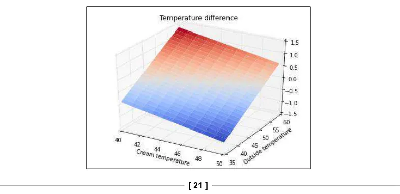
We are now ready to create a three dimensional plot of the temperature differences:
from mpl_toolkits.mplot3d import Axes3D fig = figure()
fig.set_size_inches(7,5)
ax = fig.add_subplot(111, projection='3d')
ax.plot_surface(cream_values, outside_values, temperature_differences, rstride=1, cstride=1, cmap=cm.coolwarm, linewidth=0)
xlabel('Cream temperature') ylabel('Outside temperature') title('Temperature difference')
In the preceding code segment, we started by importing the Axes3D class using the following line:
from mpl_toolkits.mplot3d import Axes3D
This class, located in the mpl_toolkits.mplot3d module, is not automatically loaded. So, it must be explicitly imported.
Then we create an object fig of the class figure, set its size, and generate an object ax that is an object of the class Axes3D. Finally, we call the ax.plot_surface() method to generate the plot. The last three command lines set the axis labels and the title.
In this explanation, we used some terms that are common in object-oriented programming. A Python object is simply a data structure that can be handled in some specialized way. Every object is an instance of a
class that defines the object's data. The class also defines methods, which are functions specialized to work with objects belonging to the class.
Notice the cmap=cm.coolwarm argument in the call to ax.plot_surface(). This sets the color map of the plot to cm.coolwarm. This color map conveniently uses a blue-red gradient for the function values. As a result, negative temperature differences are shown in blue and positive temperatures in red. Notice that there
seems to be a straight line that defines where the temperature difference transitions
from negative to positive. This actually corresponds to values where the outside temperature and the cream temperature are equal. It turns out that if the cream temperature is lower than the outside temperature, we should mix the cream into
the coffee at the coffee shop. Otherwise, the cream should be poured in the office.
Exercises
The following are some practice questions that will help you to understand and apply the concepts learned in this chapter:
• In our example, we discussed how to determine the cooling rate r. Modify the example to plot the temperature evolution for several values of r, keeping all other variables fixed.
• Search the matplotlib documentation at http://matplotlib.org to
figure out how to generate a contour plot of the temperature differences.
Our analysis ignores the fact that the cream will also change temperature as we walk. Change the notebook so that this factor is taken into account
Summary
In this chapter, we set up an IPython environment with Anaconda, accessed the IPython notebook online through Wakari, created a notebook, and learned the basics of editing and executing commands, and lastly, we went through an extensively applied example featuring the basic notebook capabilities.
In the next chapter, we will delve more deeply in the facilities provided by the notebook interface—including notebook navigation and editing facilities, interfacing with the operating system, loading and saving data, and
The Notebook Interface
The IPython notebook has an extensive user interface that makes it appropriate for the creation of richly formatted documents. In this chapter, we will thoroughly explore the notebook's capabilities. We will also consider the pitfalls and best practices of using the notebook.
In this chapter, the following topics will be covered:
• Notebook editing and navigation, which includes cell types; adding, deleting, and moving cells; loading and saving notebooks; and keyboard shortcuts
• IPython magics
• Interacting with the operating system
• Running scripts, loading data, and saving data
• Embedding images, video, and other media with IPython's rich display system
Editing and navigating a notebook
In the preceding screenshot, from the top to the bottom, we see the following components:
• The Title bar (area marked 1) that contains the name of the notebook (in the preceding example, we can see Chapter 2) and information about the notebook version
• The Menu bar (area marked 2) looks like a regular application menu
• The Toolbar (area marked 3) is used for quick access to the most frequently used functionality
• In the area marked 4, an empty computation cell is shown
Starting with IPython Version 2.0, the notebook has two modes of operation:
• Edit: In this mode, a single cell comes into focus and we can enter text, execute code, and perform tasks related to that single cell. The Edit mode is activated by clicking on a cell or pressing the Enter key.
• Command: In this mode, we perform tasks related to the whole notebook structure, such as moving, copying, cutting, and pasting cells. A series of keyboard shortcuts are available to make these operations more efficient. The Command mode is activated by clicking anywhere on the notebook, outside any cell, or by pressing the Esc key.
When we open a notebook, it's in the Command mode. Let's enter into the Edit mode in our new notebook. For this, either click on the empty cell or hit Enter. The notebook's appearance will change slightly, as shown in the following screenshot:
Notice the thick border around the selected cell and the small pencil icon on the top-right corner of the notebook menu. These indicate that the notebook is in the Edit mode.
[ 25 ]
Getting help and interrupting computations
The notebook is a complex tool that integrates several different technologies. It is unlikely that new (or even experienced) users will be able to memorize all the commands and shortcuts. The Help menu in the notebook has links to relevant documentation that should be consulted as often as necessary.
Newcomers may want to visit the Notebook Interface Tour, which is available at http://nbviewer.ipython.org/github/ipython/ ipython/blob/2.x/examples/Notebook/User%20Interface. ipynb, to get started.
It is also easy to get help on any object (including functions and methods). For example, to access help on the sum() function, run the following line of code in a cell:
sum?
Appending ?? to an object's name will provide more detailed information. Incidentally, just running ? by itself in a cell displays information about IPython features.
The other important thing to know right from the start is how to interrupt a computation. This can be done through the Kernel menu, where the kernel process running the notebook code can be interrupted and restarted. The kernel can also be interrupted by clicking on the Stop button on the toolbar.
The Edit mode
The Edit mode is used to enter text in cells and to execute code. Let's type some code in the fresh notebook we created. As usual, we want to import NumPy and matplotlib to the current namespace, so we enter the following magic command
in the first cell: %pylab inline
Press Shift + Enter or click on the Play button on the toolbar to execute the code. Notice that either of the options causes a new cell to be added under the current cell.
Just to have something concrete to work with, let's suppose we want to compute the interest accumulated in an investment. Type the following code in three successive cells:
• In cell 1, enter the following command lines:
def return_on_investment(principal, interest_rate, number_of_ years):
return principal * e ** (interest_rate * number_of_years) • In cell 2, enter the following command lines:
principal = 250 interest_rate = .034 tstart = 0.0
tend = 5.0 npoints = 6
• In cell 3, enter the following command lines:
tvalues = linspace(tstart, tend, npoints)
amount_values = return_on_investment(principal, interest_rate, tvalues)
plot(tvalues, amount_values, 'o')
title('Return on investment, years {} to {}'.format(tstart, tend)) xlabel('Years')
ylabel('Return') tstart += tend tend += tend
Now, perform the following steps:
1. Run cell 1 and cell 2 in the usual way by pressing Shift + Enter. 2. Run cell 3 by pressing Ctrl + Enter instead.
Notice that cell 3 continues to be selected after being executed. Keep pressing Ctrl + Enter while having cell 3 selected. The plot will be updated each time to display the return on the investment for a different 5-year period.
This is how the code works:
• In cell 1, we defined a function that computes the return on investment for
[ 27 ]
• In cell 2, we set actual values for the principal and interest, and then initialized
variables to define the period for which we want to do the computation. • Cell 3 computed the amount returned for a period of 5 years and plotted
the results.
• Then, the variables tstart and tend were updated. The command lines are as follows:
tstart += tend tend += tend
The effect is that, the next time the cell gets updated, time advances to the next 5-year period. So, by repeatedly pressing Ctrl + Enter, we can quickly see how the investment grows in successive 5-year periods.
There is a third way to run commands in a cell. Select cell 2 again by clicking on it. Then, press Alt + Enter in Windows or Option + Enter on a Mac. This will run cell 2 and insert a new cell under it. Leave the new cell alone for a while. We don't really need that cell, and we will learn how to delete it in the next subsection.
So, there are three ways to run the contents of a cell:
• Pressing Shift + Enter or the Play button on the toolbar. This will run the cell and select the next cell (create a new cell if at the end of the notebook). This is the most usual way to execute a cell.
• Pressing Ctrl + Enter. This will run the cell and keep the same cell selected. It's useful when we want to repeatedly execute the same cell. For example,
if we want to make modifications to the existing code.
• Pressing Alt + Enter. This will run the cell and insert a new cell immediately below it.
Another useful feature of the Edit mode is tab completion. Select an empty cell and type the following command:
print am
Then, press the Tab key. A list of suggested completions appears. Using the arrow keys of the keyboard or the mouse, we can select amount_values and then press Enter to accept the completion.
A very important feature of IPython is easy access to help information. Click on an empty cell and type:
Then, press Shift + Tab. A tooltip containing information about the linspace
function will appear. More information can be obtained by clicking on the + symbol at the top-right of the tooltip window. By clicking on the ^ symbol, the information is displayed in an information area at the bottom of the notebook.
The Tab and Shift + Tab features are the most useful ones of the notebook; be sure to use them often!
The Command mode
The number of shortcuts available in the Command mode is substantially larger than those available in the Edit mode. Fortunately, it is not necessary to memorize all of them at once, since most actions in the Command mode are also available in the menu. In this section, we will only describe some common features of the Command mode. The following table lists some of the useful shortcuts for editing cells; the other shortcuts will be described later:
Shortcut Action
Enter Activates the Edit mode
Esc Activates the Command mode
H Displays the list of keyboard shortcuts
S or Ctrl + S Saves the notebook
A Inserts a cell above
B Inserts a cell below
D (press twice) Deletes the cell
Z Undoes the last delete
Ctrl + K Moves the cell up
Ctrl + J Moves the cell down
X Cuts the content of the cell
C Copies the content of the cell
V Pastes the content of the cell below the current cell Shift + V Pastes the content of the cell above the current cell
[ 29 ]
Go ahead and try some of the editing shortcuts in the sample notebook. Here is one example that you can try:
1. Press Esc to go to the Command mode.
2. Use the arrow keys to move to the empty cell we created between cell 2 and cell 3 in the previous subsection.
3. Press D twice. This will cause the cell to be deleted. To get the cell back, press Z.
Notice that some of the shortcuts do not conform to the usual shortcuts in other software. For example, the shortcuts for cutting, copying, and pasting cells are not preceded by the Ctrl key.
Cell types
So far, we have used the notebook cells only to enter code. We can, however, use cells to enter the explanatory text and give structure to the notebook. The notebook uses the Markdown language to allow easy insertion of rich text in a cell. Markdown was created by John Gruber for plain text editing of HTML. See the project page at http://daringfireball.net/projects/markdown/basics for the basics of the syntax.
Let's see how it works in the notebook. If you created any other cells to experiment with the keyboard shortcuts in the previous section, delete them now so that the notebook only has the %pylab inline cell and the three cells where the interest computation is done.
Click on the %pylab inline cell and insert a cell right below it. You can either use the menu, or go to the Command mode (using the Esc key) and use the shortcut key B.
We now want to convert the new cell type to Markdown. There are three ways to do that. Start by clicking on the cell to select it, and then perform one of the following steps:
• Click on the notebook menu item Cell, select Cell Type, and then click on Markdown as shown in the following screenshot
• Go to the Command mode by pressing Esc and then press M
Notice that once the cell is converted to Markdown, it is automatically in the Edit mode. Now, enter the following in the new Markdown cell (be careful to leave an extra blank line where indicated):
We want to know how an investment grows with a fixed interest.
The *compound interest* formula states that:
$$R = Pe^{rt}$$
where:
- $P$ is the principal (initial investment). - $r$ is the annual interest rate, as a decimal. - $t$ is the time in years.
- $e$ is the base of natural logarithms.
- $R$ is the total return after $t$ years (including principal)
For details, see the [corresponding Wikipedia entry](http://
en.wikipedia.org/wiki/Compound_interest).
[ 31 ]
After the text is entered, press Shift + Enter to execute the cell. Instead of using the IPython interpreter to evaluate the cell, the notebook runs it through the Markdown interpreter and the cell is rendered using HTML, producing the output displayed in the following screenshot:
In this example, we use the following Markdown features:
• Text is entered normally and a new paragraph is indicated by letting an extra blank line within the text.
• Italics are indicated by enclosing the text between asterisks, as in *compound interest*.
• Formulae enclosed in double dollar ($$) signs, as in $$R = Pe^{rt}$$, are displayed centered in the page.
• An unordered list is indicated by lines starting with a dash (-). It is important to leave blank lines before and after the list.
• A single dollar ($) sign causes the formula to be typeset inline.
• Hyperlinks are specified in the following format: [corresponding Wikipedia entry]( http://en.wikipedia.org/wiki/Compound_interest).
In a Markdown cell, mathematical formulae can be entered in LaTeX, which is an extensive language for technical typesetting that is beyond the scope of this book.
Fortunately, we don't need to use the full-fledged formatting capabilities of LaTeX,
To edit the contents of a Markdown cell once it has been displayed, simply double-click on the cell. After the edits are done, run the cell using Shift + Enter to render it again.
To add structure to the notebook, we can add headings of different sizes. Let's add a global heading to our notebook:
1. Add a new cell at the very top of the notebook and change its type to
Heading 1. Recall that there are three alternatives to do this:
° By navigating to Cell | Cell Type
° Using the Cell Type dropdown on the toolbar
° Using the keyboard shortcut 1 in the Command mode
2. Enter a title for the notebook and run the cell using Shift + Enter.
The notebook supports six heading sizes, from Heading 1 (the largest) to Heading 6
(the smallest).
The Markdown language also allows the insertion of headings, using the hash (#) symbol. Even though this saves typing, we recommend the use of the Heading 1 to Heading 6 cells. Having the headings in separate cells keeps the structure of the notebook when it is saved. This structure is used by the nbconvert utility.
The following table summarizes the types of cells we considered so far:
Cell type Command mode shortcuts Use
Code Y This allows you to edit and write new code
to the IPython interpreter. The Default language is Python.
Markdown M This allows you to write an explanatory text.
Heading 1 to Heading 6
Keys 1 to 6 This allows you to structure the document
Raw NBConvert
R The content of this cell remains unmodified
[ 33 ]
IPython magics
Magics are special instructions to the IPython interpreter that perform specialized actions. There are two types of magics:
• Line-oriented: This type of magics start with a single percent (%) sign
• Cell-oriented: This type of magics start with double percent (%%) signs
We are already familiar with one of the magic command, that is, %pylab inline. This particular magic does two of the following things: it imports NumPy and matplotlib, and sets up the notebook for inline plots. To see one of the other options, change the cell to %pylab.
Run this cell and then run the cell that produces the plot again. Instead of drawing the graph inline, IPython will now open a new window with the plot as shown in the following screenshot:
This window is interactive and you can resize the graph, move it, and save it to a
Another useful magic is %timeit, which records the time it takes to run a line of Python code. Run the following code in a new cell in the notebook:
%timeit return_on_investment(principal, interest_rate, tvalues)
The output will be something like this:
100000 loops, best of 3: 3.73 µs per loop
To obtain a better estimate, the command is run 10,000 times and the runtime is averaged. This is done three times and the best result is reported.
The %timeit magic is also available in the Edit mode. To demonstrate this, run the following command in a cell:
principal = 250
interest_rates = [0.0001 * i for i in range(100000)] tfinal = 10
In the next cell, run the following command:
%%timeit returns = []
for r in interest_rates:
returns.append(return_on_investment(principal, r, tfinal))
The preceding code computes a list with the returns for 100,000 different values of the interest rate, but uses plain Python code only. The reported time for this code is displayed in the following output:
10 loops, best of 3: 31.6 ms per loop
Let's now rewrite the same computation using NumPy arrays. Run the following command in a cell:
principal = 250
interest_rates = arange(0, 10, 0.0001) tfinal = 10
In the next cell, run the following command:
%%timeit
returns = return_on_investment(principal, interest_rates, tfinal)
Now, the runtime is displayed in the following output:
[ 35 ]
When comparing the two outputs, we can see the speed gain obtained using NumPy.
To list all magics that are available, run the following command in a cell:
%lsmagic
Once you have the list of all magics, you can inquire about a particular one by running a cell with the magic name appended by a question mark: %pylab?.
This will display the information about the %pylab magic in a separate window at the bottom of the browser.
Another interesting feature is the capability to run code that is written in other languages. Just to illustrate the possibilities, we'll see how to accelerate the code using Cython, because Cython compiles Python code into C. Let's write a function that computes approximations of areas bounded by a sine curve. Here is how we
could define the function in pure Python: import math
We will approximate the area by taking the average of the left and right endpoint
rules (which is equivalent to the Trapezoidal rule). The code is admittedly inefficient
and unpythonic. Notice in particular that we use the Python library version of the sin() function, instead of the NumPy implementation. The NumPy implementation, in this case, actually yields a slower code due to the repeated conversions between lists and arrays.
To run a simple test, execute the following command in a cell:
sin_area(0, pi, 10000)
We get the following output after running the preceding cell:
1.9999999835506606
The output makes sense, since the actual value of the area is 2. Let's now time the execution using the following command:
%timeit sin_area(0, pi, 10000)
We will get the following output:
100 loops, best of 3: 3.7 ms per loop
Let's now implement the same function in Cython. Since the Cython magic is in
an extension module, we need to load that module first. We will load the extension
module using the following command:
%load_ext cythonmagic
Now, we will define the Cython function. We will not discuss the syntax in detail,
but notice that it is pretty similar to Python (the main difference in this example is that we must declare the variables to specify their C type):
%%cython cimport cython
from libc.math cimport sin
@cython.cdivision(True)
def sin_area_cython(a, b, nintervals): cdef double dx, sleft, sright cdef int i
dx = (b-a)/nintervals sleft = 0.0
sright = 0.0
for i in range(nintervals): sleft += sin(a + i * dx)
sright += sin(a + (i + 1) * dx) return dx * (sright + sleft) / 2
Test the preceding function using the following command:
sin_area_cython(0, pi, 10000)
After running the preceding function, we get the same output as earlier:
1.9999999835506608
Let's now time the function using the following command:
%timeit sin_area_cython(0, pi, 10000)
The runtime is displayed in the following output:
[ 37 ]
We see that the Cython code runs in about 30 percent of the total time taken by the Python code. It is important to emphasize that this is not the recommended way to speed up this code. A simpler solution would be to use NumPy to vectorize the computation:
def sin_area_numpy(a, b, nintervals): dx = (b - a) / nintervals
xvalues = arange(a, b, dx) sleft = sum(sin(xvalues)) sright = sum(sin(xvalues + dx)) return dx * (sleft + sright) / 2
The time after running the preceding code is displayed in the following output:
1000 loops, best of 3: 248 µs per loop
There is a lesson here; when we try to speed up the code, the first thing to try is to
always write it using NumPy arrays, taking the advantage of vectorized functions. If further speedups are needed, we can use specialized libraries such as Numba and NumbaPro (which will be discussed later in this book) to accelerate the code. In fact, these libraries provide a simpler approach to compile the code into C than using Cython directly.
Interacting with the operating system
Any code with some degree of complexity will interact with the computer's operating
system when files must be opened and closed, scripts must be run, or online data
must be accessed. Plain Python already has a lot of tools to access these facilities, and IPython and the notebook add another level of functionality and convenience.
Saving the notebook
The notebook is autosaved in periodic intervals. The default interval is 2 minutes,
but this can be changed in the configuration files or using the %autosave magic. For example, to change the autosave interval to 5 minutes, run the following command:
%autosave 300
Notice that the time is entered in seconds. To disable the autosave feature, run the following command:
We can also save the notebook using the File menu or by clicking on the disk icon on the toolbar. This creates a checkpoint. Checkpoints are stored in a hidden folder and can be restored from the File menu. Notice that only the latest checkpoint is made available.
Notebooks are saved as plain text files with the .ipynb extension, using JSON. JSON is a format widely used for information exchange in web applications, and is documented in http://www.json.org/. This makes it easy to exchange notebooks with other people: simply give them the .ipynb file, and it can then be copied to the appropriate working directory. The next time the notebook server is opened in that directory, the new notebook will be available (or the directory list can be refreshed from the dashboard). Also, since JSON is in a plain text format, it can be easily versioned.
Converting the notebook to other formats
Notebooks can be converted to other formats using the nbconvert utility. This is a command-line utility. So, to use it, open a terminal window in the directory that
contains your notebook files.
Windows users can press Shift and right-click on the name of the directory that contains the notebook files and then select Open command window here.
Open a shell window and enter the following line:
ipython nbconvert "Chapter 2.ipynb"
You must, of course, replace Chapter 2.ipynb with the name of the file that
contains your notebook. The file name must be enclosed by quotes.
The preceding command will convert the notebook to a static HTML page that can be directly placed in a web server.
An alternative way to publish notebooks on the Web is to use the site http://nbviewer.ipython.org/.
It is also possible to create a slideshow with nbconvert using the following command:
[ 39 ]
However, to get a decent presentation, we must first specify its structure in the notebook. To do so, go to the notebook and select Slide show on the Cell toolbar drop-down list. Then, determine for each cell if it should be a slide, a sub-slide, or a fragment.
To view the slide show, you need to install the reveal.js file in the same directory
as the web page containing the presentation. You can download this file from
https://github.com/hakimel/reveal.js. If necessary, rename the directory
that contains all the files to reveal.js. We are then ready to open the HTML file that contains the presentation.
It is also possible to convert notebooks to LaTeX and PDF. However, this requires the installation of packages not included in Anaconda.
Running shell commands
We can run any shell command from the notebook by starting a cell with an exclamation (!) mark. For example, to obtain a directory listing in Windows, run the following command in a cell:
!dir
The equivalent command in Linux or OS X is the following:
!ls
You can enter command lines of any complexity in the cell. For example, the
following line would compile the famous "Hello, world!" program every student of C has to try:
!cc hello.c –o hello
Of course, this will not run correctly in your computer unless you have the C compiler, cc, installed and the hello.c file with the proper code.
Instead of using shell commands directly, a lot of the same functionality is provided by magic commands. For example, a directory listing (in any operating system) is obtained by running the following command: