Time scaling internal state predictive control of a
solar plant
R. N. Silva
a, L. M. Rato
b, J. M. Lemos
caCorresponding author: DEE-FCT/UNL, 2829-516 Caparica, Portugal, [email protected], Fax.+351 212948532
bINESC-ID/Univ. ´Evora, Portugal, email: [email protected] cINESC-ID/IST, Lisboa, Portugal, email: [email protected]
Abstract
The control of a distributed collector solar field is addressed in this work, exploiting the plant’s transport characteristic. The plant is modeled by a hyperbolic type partial differen-tial equation (PDE) where the transport speed is the manipulated flow, i.e. the controller output. The model has an external distributed source, which is the solar radiation captured along the collector, approximated to depend only of time. From the solution of the PDE, a linear discrete state space model is obtained by using time-scaling and the redefinition of the control input. This method allows overcoming the dependency of the time constants with the operating point. A model-based predictive adaptive controller is derived with the internal temperature distribution estimated with a state observer. Experimental results at the solar power plant are presented, illustrating the advantages of the approach under con-sideration. Copyright c2002
Key words: Time-scaling, adaptive control, predictive control, solar energy, distributed
plant.
1 INTRODUCTION
In the approach here presented, the internal dynamics are taken into account and the control law includes feedback terms by means of a state observer. Furthermore, the introduction of the internal state estimation allows the controller to damp the internal oscillations that arise from the cancelation of anti-resonant modes.
Although the authors, among other researchers, have participate on the develop-ment of several controllers for this plant using adaptive predictive control tech-niques (Coito et al., 1997; Silva et al., 1998; Silva et al., 1997; Rato et al., 1997; Pickhardt and Silva, 1998), i.e. without any a priori knowledge about the plant, in this work, the goal was to increase performance by the development of an adaptive predictive controller embedding in its design the relevant physical characteristics of the plant. The ACUREX field used in these experiments is described in avail-able literature (Camacho et al., 1992; Camacho et al., 1988) and has motivated a wide range of research work on more sophisticated controllers of which (Bar ˜ao et al., 2002; Berenguel and Camacho, 1995; Camacho et al., 1994; Camacho et al., 1994; Camacho, Berenguel and Rubio, 1997; Camacho et al., 1992; Camacho and Berenguel, 1997; Coito et al., 1997; Carotenuto et al., 1985; Carotenuto et al., 1986; Johansen et al., 2000; Johansen et al., 2002; Lemos, Rato and Mosca, 2000; Meaburn and Hughes, 1994; Orbach et al., 1981; Rorres et al., 1980; Rubio et al., 1995; Rubio et al., 1996; Silva et al., 1997) are significant examples.
In this plant, the main sources of disturbances are measured and its dynamic be-havior depends strongly on its geometry (available). This allows us to derive an ac-curate model that is described by a partial differential equation (PDE). The plant is characterized by: non-linearity caused by the dependency of bandwidth and static gain with flow (the manipulated variable); fast accessible disturbances (solar ra-diation with sudden clouds); time varying dynamics with the daily and annually cycles, and pluvial cycles that modify the reflectivity of the mirrors; and sudden plant changes when groups of collectors are entering/exiting solar track.
Since the controller is to be implemented in a digital computer, the dynamic de-pendency on flow can be overcome by time-scaling, replacing the elements of time (sampling period) by elements of volume. This results in a discrete linear model with variable sampling period dependent on the imposed flow. Plants, such as rolling mills, conveyor belts or fluids in pipes, can be transformed with time-scaling ( ˚Astr¨om and Wittenmark, 1984). Plants of this class may be controlled with advantage using the method reported here, which takes into consideration the de-pendency of the time-scaling on the manipulated variable.
From the Adaptive Predictive Control point of view, the loss of generality of the results here presented is compensated by the possibility of extending them for the class of systems modeled by similar equations (PDEs), e.g. heat-exchangers, road traffic, river pollution, etc.
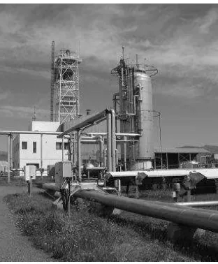
Fig. 1. Solar collectors (one of the twenty rows).
Fig. 2. Oil storage tank.
non-linear model is described. Section 3 describes the controller design. In section 4, some experimental results on the real plant are shown and some conclusions are drawn in section 5.
2 THE SOLAR PLANT
2.1 PLANT DESCRIPTION
The ACUREX field of the Plataforma Solar de Almer´ıa (PSA) is located in the south of Spain and consists of 480 distributed solar collectors, arranged in 10 loops along an east-west axis (fig. 1). The collector has a reflective cylindrical parabolic surface, in order to concentrate the incident solar radiation on a pipe located on the surface focal line.
Fig. 3. Radiation sensor with 2 d.o.f.
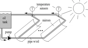
mirrors temperature
sensors
pump
pipe w/oil oil
tank
Fig. 4. Process schematic.
The controlled variable is computed from the average values of an array of 10 temperature sensors located at the output of each loop.
Due to safety reasons, the oil flow is limited between 2.0 and 10.0 liters per second. The heated oil from the collector field, stored in the tank, can be used e.g. for the production of electrical energy or for the operation of a desalination plant.
The field is equipped with a tracking system by which the mirrors can rotate parallel to the axis of the receiving tube, in order to follow the sun in height throughout the day. There is a temperature sensor located at the input of the field, measuring the temperature of the oil entering the active part (mirrors). A 2 d.o.f. solar radiation sensor, able to track the sun, is also available to measure the total incident radiation (fig.3). From this measure, it is possible to compute the corrected radiation (i.e. the effective radiation heating the oil), using an algorithm with the actual day and time.
Simulation results show that this plant cannot perform well under all operating systems with linear methods (Bar˜ao et al., 2002).
2.2 PLANT MODEL
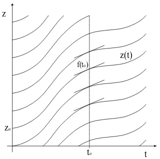
z
t
z(t)
zo
to
f(to)
Fig. 5. Characteristic curves whenw(t)≡0.
which models transport phenomena equation with variable transport speed and a distributed source:
∂y(z, t)
∂t +
f(t)
A
∂y(z, t)
∂z = Γw(t) (1)
whereyis the temperature distribution along spacezand timet;fis the volumetric flow and w is the effective solar radiation. The parameter Γ = (Dηo)/(ρASf) (whereDis the mirrors width,ηois the optical efficiency,Ais the transversal pipe section area,Sf is the specific thermal capacity of the oil andρ is the oil density approximated by a constant) has been estimated using real plant data.
Considering first the case when the r.h.s. of eq. (1) is zero, i.e.w(t)≡ 0, the PDE admits then solutions given in the implicit form
y(z, t) = φ
z− 1
A
t
Z
t0
f(σ)dσ
(2)
whereφ(z)is the initial (t =t0) temperature distribution. This means that the ini-tial temperature profile moves, with its shape unchanged, in a convective transport defining paths (characteristic curves)z =z(t)along which the value ofydoes not vary with respect to time (fig. 5).
Mathematically, we are looking for a path z(t)(known as a characteristic curve), parameterized by time, such that
dy(z(t), t)
which, by the chain rule, is equivalent to
∂y(z, t)
∂z dz dt +
∂y(z, t)
∂t = 0 (4)
Ifysolves equation (3) then this would be satisfied provided that
dz dt =
f(t)
A (5)
This ODE has solutions of the form
z(t) = 1
A
t
Z
t0
f(σ)dσ+z0 (6)
In the general case of equation (1), since the r.h.s. is independent ofy, the solution can again be found using the chain rule of derivation to integrate the collected solar radiation along the characteristic curve:
dy(z(t), t)
dt = Γw(t) (7)
yielding for the temperature at the outputz =L
y(L, t) = Υy(0, t0) + Γ
t
Z
t0
w(σ)dσ (8)
with the transport timeτ =t−t0, given by
t
Z
t−τ
f(σ)dσ =L A=V (9)
whereV is the total collector volume. The parameter Υin equation (8) has been introduced in order to take the losses into account. Since the losses in this plant are not significant, this parameter arises as a simplification of the problem (the losses depend on the residence time i.e. the flow). In (Pickhardt and Silva, 1998) a different approach for obtaining the model given by equations (8) and (9) is shown, based on energy balances.
The equations (8) and (9) allow us to establish a steady-state relationship among the I/O temperature gain,∆T , the solar radiationw¯and the flow f¯as
∆T = (ΓV)w¯¯
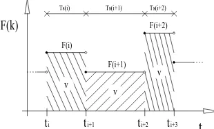
ti ti+1 ti+2 ti+3 t
v
v v
Ts(i) Ts(i+1) Ts(i+2)
F(k)
F(i)
F(i+1) F(i+2)
Fig. 6. Relation between the flow and sampling period.
this relation will be useful further on in the interpretation of the resulting control law.
2.3 TIME-SCALED DISCRETIZATION
Considering again equations (8) and (9), and using elementary volumes instead of elementary time intervals (sampling period) on a discretization procedure, the collector volume,V, is divided innsmaller equal volumes,ν. Since the controller will be implemented in a digital computer, a zero order hold (ZOH) is considered for the flow command. Choosing the sampling period,TS, for each discrete time epoch,k, such that the product of the flow value by the sampling period results in the elementary volume (fig. 6), i.e.
ν = V
n
f(k)×Ts(k) = ν (11)
Then, equation (9) implies that
n
X
i=1
Ts(k−i) =τk (12)
where τk stands for the I/O transport delay (through volume V), in seconds, for the fluid element present at the output at time instantk. The discrete time radiation signal can be computed from the continuous one with a forward average at timek
as
w(k) = 1
Ts(k) tk+1
Z
tk
w(σ)dσ (13)
w ( k ) α.R(t) y(k)
ν
Flo w - F (k)
ν ... ν ν
x (k)1 x (k)2 x (k)n-2 x (k)n-1 x (k)=y(k)n
Fig. 7. State temperatures.
period (11) yielding, in discrete time,
xj(k+ 1) =βxj−1(k) + Γw(k)Ts(k) (14)
whereβ ≈ 1is a loss parameter such thatβn = Υandx
i(k)is the oil temperature at the output of the subvolumei(see fig. 7) at the (discrete) time instantk . Using (11) this can be written as
xj(k+ 1) =βxj−1(k) +α
w(k)
f(k) j = 1· · ·n
y(k) =xn(k)andx0(k) =v(k) (15)
whereα= Γνis the solar energy capture efficiency for a subvolumeν.
Gathering these equations in a state-space frame yields
X(k+ 1) =
−1 −0.8 −0.6 −0.4 −0.2 0 0.2 0.4 0.6 0.8 1 placed at the origin resulting from the transport dynamics.
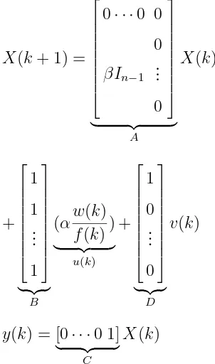
The zeros of the discrete plant’s transfer function are given by the roots of the polynomial:
zn−1+βzn−2+· · ·+βn−2z+βn−1 (17)
These zeros are distributed along a circle of radiusβ(fig. 8):
z =β ej2nπi, i= 1· · ·(n−1) (18)
This anti-resonance behavior is not due to the discretization procedure, since it is also present in the continuous model.
The controllability (foruandwinputs) and observability matrices are given by:
O =
0 · · · 0 1
..
. 0 β 0
0 ··· 0 ...
βn−1 0 · · · 0
(21)
and thus the system is fully controllable and fully observable.
3 THE CONTROLLER
3.1 PREDICTIVE CONTROLLER DESIGN
After expressing the plant in a classical state-space frame, with verified controlla-bility and observacontrolla-bility, the control should arise as a straightforward step, choosing the desired eigenvalues distribution and determining the state feedback gain vector using some standard method.
Hereafter, a predictive multistep cost function is proposed in order to set, using the control horizon, the amount of fluid inside the volume that should be considered to compute the control action. It is to be expected that a cost function, covering all the collector volume, will result in a control action much smoother than if the controller is only looking for the pipe’s last section.
Considering the following cost function (T < n):
JT = T
X
i=1
n ˜
y2(k+i) +ρu2(k)o (22)
wherey˜(k) =y(k)−r(k)is the control error withrbeing the reference to track.
The future values of the output error are given by
˜
y(k+i) = CX(k+i)−r(k+i)
X(k+i) = AiX(k) +C
Bi[u(k+i−1)· · ·u(k)] T
+CDi[v(k+i−1)· · ·v(k)]
with
If the minimization of (22) is made under the assumption of constant control action and constant input temperature over the control horizon, i.e.,
u(k) =· · ·=u(k+i−1) (27)
v(k) =· · ·=v(k+i−1)
then the terms of the r.h.s. of (23) are given by:
CAiX(k) =β
minimiza-tion of (22) yields a control acminimiza-tion:
u(k) = (
PT
i=1λi)r(k)−PiT=1λiβixn−i(k)
PT
i=1λ2i +ρ
(29)
whereλi = 1 +β+· · ·+βi−1. Then, the flow applied to the field is computed from
f(k) = αw(k)
u(k) (30)
and the length of the sampling period at epochkis given by
Ts(k) =
ν
f(k) (31)
The control law given by equation (29) has an interesting physical interpretation. Consideringρ = 0 (no control penalty) and β = 1 (no losses); with T = 1 the control law reduces to
u(k) = αw(k)
f(k) =
r(k)−xn−1(k)
1 (32)
Comparing this control law with the steady-state relation from equation (10), it is seen that the control establishes the necessary flow to guarantee that the oil at the one before last (n−1) sub-volume will reach the output, in the next sampling period, being equal to the reference.
With larger values of T (again with ρ = 0 and β = 1), the control law can be rewritten as
u(k) = αw(k)
f(k) =
(r(k)−xn−1(k)) + 4×(r(k)−x
n
−2(k))
2 +· · ·+T
2 ×(r(k)−xn
−T(k))
T
1 + 4 +· · ·+T2 (33)
−1 −0.8 −0.6 −0.4 −0.2 0 0.2 0.4 0.6 0.8 1
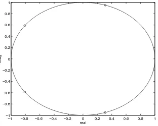
Fig. 9. Closed-loop system eigenvalues (n=4).
0 10 20 30
Fig. 10. Simulation results (n=5; T=1 and T=2).
It is remarked that the condition of keeping the control action constant along the horizon arises, not only from the simplicity thereby introduced in the minimization procedure, but also because it should be the best strategy to cope with the existence of anti-resonance modes. Due to the Finite Impulse Response (FIR) structure of the model, the best control strategy (assuming constant radiation) should be to apply a step, with the adequate amplitude, and wait for the new equilibrium point to be reached. This strategy, in open-loop, would provide a ramp temperature profile inside the collector pipe, with the final temperature equal to the desired one. Now, with a receding horizon strategy, only the first control action is applied to the plant and the minimization is repeated over the next time sample.
Since the horizonT is discrete and the sampling periodTs(k)depends on the flow, the value ofT establishes, not the time horizon into the future, but the amount of oil inside the collectors that is important for the computation of the control action. Figure 9 shows the distribution of the resulting eigenvalues forT = 1 to 4when
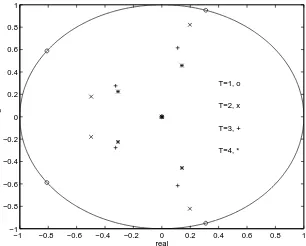
0 10 20 30
Fig. 11. Simulation results (n=5; T=3 and T=4).
−1 −0.8 −0.6 −0.4 −0.2 0 0.2 0.4 0.6 0.8 1
Fig. 12. Observer eigenvalues (n=20).
3.2 OBSERVER DESIGN
In the ACUREX field, the measures of the internal oil temperature are not available. To overcome this, a state observer has been implemented with the observer gain given by
which is equivalent to a progressive linear correction along the pipe. Then, the observer characteristic polynomial is given by
P(λ) =|λI −A+L C|
12.5 13 13.5 14 14.5 15 15.5 200
220 240 260 280 300
T [C]
ACUREX, 28−06−2001
12.5 13 13.5 14 14.5 15 15.5
2 4 6 8 10
F [l/s]
t [h]
50 deg C 50 deg C
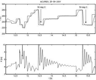
Fig. 13. Exp. 1 Output temperature and reference (top); and field flow (bottom).
4 EXPERIMENTAL RESULTS
4.1 EXPERIMENTAL CONDITIONS
The following experiments have been made at PSA in June 2001.
An important practical issue is to select the number of collector divisions,n. This value will establish, with the range of allowed flows, the sampling period range. The total field volume for the active part is around1800liters. A value ofn = 20
was chosen in order to get a sampling period between
Tsmin =
1
fmax
V
n = 9s and T
max
s =
1
fmin
V
n = 45s
In previous works with this plant, values of the sampling period between 15s and 39s have been used.
4.2 EXPERIMENT 1.
This experiment was performed with T = 8, and gives emphasis to the ability of the time-scaled predictive controller to make set-point temperature changes of
50◦C, overcoming the non-linearity that results from the sudden change in the flow
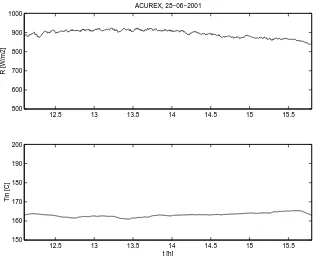
value. In figure 13, the output temperature is presented with its reference on the top plot and it is possible to observe the flow signal on the bottom one. Figure 14 shows the solar radiation (top) and the input temperature (bottom).
12.5 13 13.5 14 14.5 15 15.5 500
600 700 800 900 1000
R [W/m2]
ACUREX, 28−06−2001
12.5 13 13.5 14 14.5 15 15.5
150 160 170 180 190 200
Tin [C]
t [h]
Fig. 14. Exp. 1. Solar radiation (top); and input temperature (bottom).
12.5 13 13.5 14 14.5 15 15.5
200 220 240 260 280 300
T [C]
ACUREX, 29−06−2001
12.52 13 13.5 14 14.5 15 15.5
4 6 8 10
F [l/s]
t [h]
Fig. 15. Exp. 2 Output temperature and reference (top); and field flow (bottom).
12.5 13 13.5 14 14.5 15 15.5
500 600 700 800 900 1000
R [W/m2]
ACUREX, 29−06−2001
12.5 13 13.5 14 14.5 15 15.5
150 160 170 180 190 200
Tin [C]
t [h]
Fig. 16. Exp. 2. Solar radiation (top); and input temperature (bottom).
4.3 EXPERIMENT 2.
11.5 11.55 11.6 11.65 11.7 11.75 11.8 11.85 11.9 200
220 240 260 280 300
T [C]
ACUREX, 27−06−2001
11.50 11.55 11.6 11.65 11.7 11.75 11.8 11.85 11.9 2
4 6 8 10
F [l/s]
t [h]
Fig. 17. Exp. 3 Output temperature and reference (top); and field flow (bottom).
11.5 11.55 11.6 11.65 11.7 11.75 11.8 11.85 11.9 180
190 200 210 220 230 240 250 260 270 280
Tin, Xi, Tout [C]
ACUREX, 27−06−2001
t [h]
Fig. 18. Exp. 3. Input/output temperatures and estimated internal temperature.
4.4 EXPERIMENT 3.
Although it is not very beneficial to the field’s pump, an experiment withT = 1
was performed, for a period of half an hour, to confirm the cancelation effect. In figure 17 the output temperature is presented with its reference on the top plot and it is possible to observe the flow signal on the bottom one. Figure 18 shows again the output temperature, the estimated temperature in the middle of the collector and the input temperature.
Attention should be payed to the fact that both the flow and the internal tempera-ture present strong oscillations compared to the output temperatempera-ture with only15◦C
amplitude.
5 CONCLUSIONS
manip-ulated variable, the flow. The algorithm has been applied to the real plant and the results are presented in this paper.
This concept is not restricted to this particular field (the ACUREX). Any solar field using this concept of manipulating flow to change the residence time inside the collector can overcome the time constants dependence on flow with this kind of transformation.
Acknowledgements
Part of this work has been done under the project POSI/1999/SRI/36328 (AM-BIDISC) and under IIIrd EC Framework Program. The experiments were supported by EC-DGXII under the IHP-ARI (5FP). The authors are thankful to the excellent and friendly support provided by all the staff at Plataforma Solar de Almer´ıa.
References
˚
Astr¨om, K., and B. Wittenmark (1989). Adaptive Control. Addison Wesley.
Bar˜ao, M.; J. M. Lemos and R. N. Silva (2002). Reduced complexity adaptive control of a distributed collector solar field. J. Proc. Control, ˙bf 12, 131-141.
Berenguel, M. and E. Camacho (1995). Frequency based adaptive control of systems with antiressonance modes. Prep. 5th IFAC Symp. Adaptive Systems in Control and Signal
Processing. Budapest, Hungary, 195-200.
Camacho, E.; F. Rubio and J. Gutierez (1988). Modelling and simulation of a solar power plant with distributed collector system, IFAC Symp. on Power Systems Modelling and Control Applications, Brussels.
Camacho, E.; F. Rubio and F. Hughes (1992). Self-tuning control of a solar power plant with a distributed collector field, IEEE Control Systems Mag., 72-78.
Camacho, E. F., M. Berenguel, C. Bord ´ons (1994). Adaptive Generalized Predictive Control of a Distributed Collector Field, IEEE Trans. Contr. Syst. Tech., 2, 4, 462-467.
Camacho, E. F., M. Berenguel and F. Rubio (1994). Application of a gain scheduling generalized predictive controller to a solar power plant, Control Eng. Practice 2, 2, 227-238.
Camacho, E., M. Berenguel and F. Rubio (1997). Advanced Control of Solar Plants. Springer-Verlag.
Carotenuto, L., M. La Cava and G. Raiconi (1985). Regular design for the bilinear distributed parameter of a solar power plant. Int. J. of Systems Science, 16, 885-900. Carotenuto, L., M. La Cava, P. Muraca and G. Raiconi (1986). Feedforward control for the
distributed parameter model of a solar power plant. Large Scale Systems, 11, 233-241. Coito F., J.M. Lemos, R. N. Silva and E. Mosca (1997). Adaptive control of a solar energy plant: exploiting acceptable disturbances. Int. Journal of Adaptive Control and Signal
Processing, 11, 327-342.
Johansen, T. A., K. Hunt and I. Petersen (2000). Gain scheduled control of a solar power plant. Control Eng. Practice, 8, 1011-1022.
Johansen, T. A. and C. Storaa (2002). Energy-based control of a solar collector field.
Automatica, 38, 1191-1199.
Lemos, J. M.,; L. M. Rato and E. Mosca (2000). Integrating predictive and switching control: Basic concepts and an experimental case study. In Nonlinear Model Predictive
Control, F. Allg ¨ower and A. Zheng eds. Birkh¨auser Verlag, Basel, Boston, Berlin,
181-190.
Meaburn, A. and F. M. Hughes (1994). Prescheduled Adaptive Control scheme for ressonance cancellation of a distributed solar collector field. Solar Energy, 52(2):155-166.
Orbach, A.; C. Rorres and R. Fischl (1981). Optimal control of a solar collector loop using a distributed-lumped model. Automatica, 27, 3, 535-539.
Pickhardt, R., and R. N. Silva (1998). Application of a nonlinear predictive controller to a solar power plant. Proc. 1998 IEEE-CCA, Trieste, Italy.
Rato, L.; R. N. Silva, J.M. Lemos e F. J. Coito (1997). Multirate MUSMAR cascade control of a distributed collector solar field. European Control Conference 97, Brussels, Belgium.
Rorres, C.; A. Orbach and R. Fischl (1980). Optimal and suboptimal control policies for a solar collector system. IEEE Trans. Autom. Control, AC-25, 6, 1085-1091.
Rubio, F.; M. Berenguel and E. Camacho (1995). Fuzzy logic control of a solar power plant. IEEE Trans. on Fuzzy Systems, 3, 4, 459-468.
Rubio, F., F. Gordillo and M. Berenguel (1996). LQG/LTR Control of the Distributed Collector Field of a Solar Power Plant. Prep. IFAC Symp. Adaptive Systems in Control
and Signal Processing, 335-340, Glasgow, Scotland.
Silva, R. N., L. M. Rato, J. M. Lemos and F. Coito (1997). Cascade control of a distributed collector solar field. J. Process Control, 7, 2, 111-117.
Silva, R. N. , N. Filatov, J. M. Lemos and H. Unbehauen (1998) Feedback/Feedforward Dual Adaptive Control of a Solar Collector Field. Proceedings of the 1998 IEEE-CCA, Trieste, Italy.
Silva, R. N. (1999). Time-scaled predictive controller of a solar power plant. Proc.
Silva, R. N. and J.M. Lemos (2001). Adaptive control of transport systems with non-uniform sampling. European Control Conference 01, Oporto, Portugal.
Silva, R. N., L. M. Rato e J. M. Lemos (2002). Observer based nonuniform sampling predictive controller for a solar plant. XV IFAC World Congress, Barcelona, Spain. Takahashi, Y., C. Chang, D. Auslandender (1971). Parametere-instelung bei linearen