C
–
1
Modified Genetic Algorithm to Solve Time-varying Lot Sizes
Economic Lot Scheduling Problem
Bethany Elvira1, Yudi Satria2, dan Rahmi Rusin3
1
Student in Department of Mathematics, University of Indonesia, Depok, Indonesia e-mail : [email protected]
2
Lecturer in Department of Mathematics, University of Indonesia, Depok, Indonesia e-mail : [email protected]
3
Lecturer in Department of Mathematics, University of Indonesia, Depok, Indonesia e-mail : [email protected]
Abstract
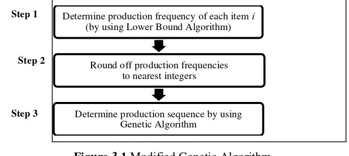
Economic Lot Scheduling Problem (ELSP) is the problem of scheduling several items on a single machine in order to meet the demand without any backorder, so as to minimize the total cost (sum of inventory holding cost and setup cost). In this problem, a product is made from combination of some types of items. The purpose of solving ELSP is to determine the duration of processing same item (called as run length or lot size) and determine the sequence of the lots (called as production sequence) that can minimize the total cost. One of the ELSP approaches is Time-varying Lot Sizes Approach, which is an approach which different lot sizes is possible for any item in the production sequence. There are three main steps to solve Time-varying Lot Sizes ELSP: (1) Determine the production frequency of each item; (2) Round-off the production frequency of each item; (3) Determine the production sequence which minimizes the total cost. Time-varying Lot Sizes ELSP is known as NP-hard problem and there are numerous research on heuristic algorithms to solve this problem. This paper proposes Modified Genetic Algorithm which is a modification of Hybrid Genetic Algorithm [3] and Two-Level Genetic Algorithm (Moon & Choi, 2002). Numerical experiments show that Modified Genetic Algorithm outperforms
Dobson’s heuristic [4] and has the same result with Hybrid Genetic Algorithm. Moreover, Modified Genetic Algorithm could have shorter computation time than Two-Level Genetic Algorithm because in Modified Genetic Algorithm there is only one level of Genetic Algorithm.
1.
Introduction
In industry, it is a common thing to produce several types of items on a single machine. For example, a machine which products some different stampings on the same press line [2].
A product is produced by combining several types of items. Machine only can produce one item at a time and the duration of processing the same item called as run length or lot size. Before producing a different item, there is setup process so that there are setup time and setup cost for each type of item. Hence there is a need to schedule the setup and production process, called as production scheduling problem.
In production scheduling problem, there is inventory level which is stock on hand subtracted with backorder (items which are demanded but not yet produced) (Axsäter, 2006, page 46). In the problem explained in this paper, backorder is not allowed so that there is inventory holding cost. Besides that, in this problem the demand rate and production rate are constant.
the approach methods: Common Cycle Approach, Basic Period Approach, and Time-varying Lot Sizes Approach. The last approach method is the most complicated problem, but its solution is the most optimal among the other methods [3]. Therefore, this paper tries to solve Time-varying Lot Sizes ELSP.
2.
Literature Review on Time-varying Lot Sizes ELSP
Data Parameters:
: Production time required for the production of item at position j : Idle time after the production of item at position j
: Cycle length (units in days)
: Cycle length of item i (units in days)
: Position in a given sequence from k, up to but not including the position in the sequence where item is produced again
In this problem, there is a single machine which has to produce m different satisfied and the total cost can be minimized. The cycle can be repeated over time and the demand can be fully satisfied.
Define
with is the long-run proportion of time available for setup [5]. Dobson (1987) showed that if > 0, then any production sequence can be converted into a feasible schedule.
The complete formulation of Time-varying Lot Sizes ELSP:
Constraint (2.3) states that the production time has to be enough for each item i to meet its demand over the cycle, with is the lot size of item i. Constraint (2.4) limits the item’s production rate, which the demand rate has to be satisfied until that item can be produced again in the next cycle. Constraint (2.5) ensures that cycle length T is equal to the summation of production time, setup time, and idle time for all items produced in cycle.
3.
Modified Genetic Algorithm
Time-varying Lot Sizes ELSP is known as NP-hard problem and there are numerous research on heuristic algorithms to solve this problem. Until now, there are two types of Genetic Algorithm to solve Time-varying Lot Sizes ELSP:
Table 3.1 Comparison between Hybrid Genetic Algorithm and Two Level Genetic Algorithm
HybridGenetic Algorithm[5] Two LevelGenetic Algorithm [3]
Advantages
The result is better than Dobson’s
heuristic (1987) because this method uses Genetic Algorithm to determine the production sequence.
Genetic Algorithm is not only used to determine the production sequence, but also to determine production frequency (rounding off production frequency optimization).
Disadvantages
This method only takes the result from rounding off production frequencies to nearest integers for computing the production sequence.
In this method, Genetic Algorithm is executed for two levels or two times so that it could lead to a longer computation time.
This paper proposes Modified Genetic Algorithm which is a modification of Hybrid Genetic Algorithm and Two-Level Genetic Algorithm. This section explains three steps in Modified Genetic Algorithm to solve Time-varying Lot Sizes ELSP frequency of each item i by solving Lower Bound Model. Bomberger (1966) proposed this model when methods to obtain optimal solution of ELSP were not yet discovered.
Bomberger determine the lower bound of the optimal solution in order to compare available feasible solutions.
The purpose of Lower Bound Algorithm is to determine production frequency of each item i under a constraint on the machine’s capacity.
subject to
The objective function and the constraint set in (3.1) and (3.2) are convex in the (Chung & Chan, 2012). The optimal points of the model are the points which satisfy Karuh-Kuhn-Tucker (KKT) conditions as in
subject to , complementary slackness with , where
Moon, Silver, & Choi (2002) proposed Lower Bound Algorithm to obtain optimal points. These are the following procedures.
Step 1: Check if gives an optimal solution Find s by using equations: .
If , then are optimal and stop, otherwise go to step 2.
Step 2: Start with an arbitrary .
Step 3: Compute for each item. Step 4: If , reduce . Go to step 3.
If , increase . Go to step 3. If , stop. The s are optimal.
Let the optimal cycle length for item i in the Lower Bound model is and let represent the production frequency for item i. Then is obtained by following:
3.2 Round off Production Frequency
The production frequencies obtained in (3.5) are decimals. Therefore, the purpose of Step 2 in Modified Genetic Algorithm is to round off the production frequency, so that the result can be applicable in real life industry.
Dobson (1987) made a heuristic method to determine the production sequence by previously rounding off the production frequencies to power-of-two integers. Roundy (1989) showed that this method could raise additional costs up to 6%. Although the additional costs are not too big, but it would be better if there is another round off method to minimize the total cost [5]. This paper doesn’t use Dobson’s heuristic to determine the production sequence. Therefore, it is not necessary to round off the production frequencies to power-of-two integers. This paper follows method from Moon, Silver, & Choi (2002), which is rounding off the production frequencies into
(3.1)
(3.2)
(3.3)
(3.4)
nearest integers, because it has been shown that solution obtained from their method is better than the solution obtained by rounding off to power-of-two integers.
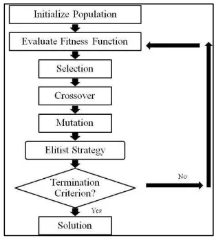
3.3 Genetic Algorithm to Determine Production Sequence
Steps in Genetic Algorithm to determine production sequence described in the following Figure 3.2.
Figure 3.2 Genetic Algorithm to Determine Production Sequence
3.3.1 Chromosome Representation and Initialize Population
For example, there are five different items that have to be produced and the result from Step 2 in Section 3.2 is can seen in the below table.
Table 3.2 Production Frequency
Item 1 2 3 4 5
Production Frequency 2 2 3 3 1
In this paper, chromosome represents production sequence and each gene in the chromosome represents the index of an item. Chromosome length is the sum of the production frequencies. In this example, the sum of the production frequencies = 2+2+3+3+1 = 11, so that the chromosome length is 11. At first the optimal production sequence is unknown, so the first step that can be conducted is allocating each item in the production sequence consecutively from left to right based on each item’s production frequency (Table 3.3). This method was proposed by Moon, Silver, dan Choi (2002). The result of this first step is called as initial chromosome.
Table 3.3 Initial Chromosome
Position 1 2 3 4 5 6 7 8 9 10 11
Item 1 1 2 2 3 3 3 4 4 4 5
After that, create a population which contains chromosomes as the result of sequence randomization of initial chromosome. This sequence randomization is under condition that each chromosome has to be different with each other. This population becomes the initial population.
3.3.2 Fitness Function Evaluation
is the fitness value of its corresponding chromosome. In order to obtain the total cost, Dobson (1987) manipulated Time-varying Lot Sizes ELSP formulation into matrix form. These are the following notations used in this manipulation.
D is a diagonal matrix with
P is a diagonal matrix with
L is a 0-1 matrix whose rows are the incidence vectors of the index sets
and is the transpose of e, i.e.
t is a column vector whose elements are production time of item produced on position j =1, …, n and is the transpose of t
s is column vector whose elements are setup time of item on position j =1, …, n
u is column vector whose elements are idle time of item on position j =1, …, n
A is column vector whose elements are setup cost of item on position j =1, …, n
T is a number which indicates cycle length
By using those notations, the problem formulation of Time-varying Lot Sizes ELSP in Section 2 becomes:
subject to
The following theorem determines when the ELSP formulated in Section 2 has a feasible solution.
Theorem 3.1 Let f be a given sequence and fixed idle times ( ). Then there exists a feasible set of production times t if and only if .
[4]
If Theorem 3.1 is satisfied, then there exists feasible set of production time t which can be obtained by manipulating equation (3.7):
From production sequence f, determine matrix P, matrix L, and setup time s to obtain production time t in equation (3.9). After that, substitute production time t into equation (3.8) to obtain cycle length T. And then matrix D and A can be obtained and substitute D, A, t and T into objective function (3.6):
3.3.3 Selection
Selection method used in this paper is Roulette Wheel Selection which is the same method used by Chung dan Chan (2012) and Moon, Silver, & Choi (2002).
The first step of this method is to determine relative fitness from each chromosome. Relative fitness from ath chromosome:
(3.6)
(3.7) (3.8)
(3.9)
where c is population size
The next step is determining cumulative fitness from each chromosome and mapping those chromosomes consecutively in a line segment so that each segment has same size with its fitness size. After that, generate random number as much as the number of the chromosomes. Chromosome which has a segment in the random number’s region will be selected [6].
3.3.4 Crossover
Crossover method used in this paper is Two Point Crossover which is the same method used by Chung dan Chan (2012). In this method, there are two positions randomly selected which later called as upper point and lower point. These are the procedures to do Two Point Crossover.
Step 1: Generate p, which is a random number between 0 and 1.
Step 2: If p < crossover rate, then the corresponding chromosome is selected to crossover and selected to get into the parent population. Otherwise, chromose isn’t selected to crossover.
Step 3: Check the number of chromosomes in parent population obtained from step 2. If
the number is odd, the last chromosome is deleted from parent population. If the
number is even, go to step 4.
Step 4: Take two chromosomes consecutively from parent population. For each pair of chromosomes, do step 5 until step 8.
Step 5: Generate 2 random numbers for upper point and lower point, those numbers have
to be located in interval [1, number of genes in one chromosome]. If upper point <
lower point, then exchange the position.
Step 6: Create two offspring which inherit all genes from each parent. After that, exchange gene between offspring at lower point. And then validate gene. Step 7: Do step 6 for upper point
Step 8: Insert two offspring chromosomes into crossover population.
3.3.5 Mutation
Just like crossover step, mutation method in this paper follows the same method by Chung and Chan (2012). These are the procedures to do mutation.
Step 1: Calculate number of genes in the population.
Step 2: Generate p=random number within range [0,1] as much as the number of genes. Step 3: If p < mutation rate, then do mutation on that gene, do mutation within the
range [1, maximum item’s index]. Otherwise, that gene isn’t mutated. Step 4: Validate gene in chromosome which has mutated genes.
3.3.6 Elitist Strategy
Elitist strategy used by Chung dan Chan (2012) is replacing the worst 20% of the chromosomes with the best chromosomes from selection, crossover, and mutation. In Time-varying Lots Sizes ELSP, the best chromosome is the chromosome which has
the smallest fitness value. The result of elitist strategy becomes chromosomes for next generation.
4.
Computational Experiments
Implementation of Modified Genetic Algorithm is executed by using Python 2.7. The program made in Eclipse 4.2.2 with plug in Pydev. This program is executed on computer which has specifications: Processor Intel® Core™ i5-3317U @ 1.70GHz, RAM 4096 MB, and Windows 8 Pro 64-bit. Program explained in this paper is used to solve Mallya’s problem [7] which can be seen in Table 4.1. This problem assumes idle time (u) = 0.
Table 4.1 Mallya’s Problem [7]
i
1 1800 474 0.2 80 0.00379 0.001327
2 2500 413 0.35 140 0.00252 0.000882
3 4000 528 0.15 60 0.00391 0.001369
4 3200 985 0.25 100 0.00282 0.000987
5 1500 166 0.15 60 0.00108 0.000378
[ is standard cost with holding cost or ]
There are some experiments done in this paper by changing parameters of Genetic Algorithm: crossover rate, mutation rate, population size, and maximum generation. In order to determine the best solution of Modified Genetic Algorithm, the result of Lower Bound Algorithm is used as a reference where the result of Mallya’s problem is total cost = $57.73. As the solution more approaching the Lower Bound Algorithm’s result, the better the solution.
4.1 Experiment on Different Crossover Rates and Mutation Rates
The first experiment is conducted by using population size = 100 and maximum generation = 200. This experiment uses the same crossover rate and mutation rate: 0.2, 0.3, 0.1, and 0.5.These rates are chosen based on the experiment by Chung and Chan (2012). The result of the first experiment can be seen in the following figure.
Figure 4.1 The Result of Experiment on Different Crossover and Mutation Rates
Graph in Figure 4.1 indicates the transformation of minimum total cost or best fitness value towards generations. By using crossover rate = 0.5 and mutation rate = 0.5, we can obtain the optimal solution with shortest time (fastest convergence time).
From the Figure 4.1, it can be seen that although this experiment uses different crossover rates and mutation rates, the final result still converged to one solution, which is total cost = $60.91, with details:
generation
tot
a
l
co
f = (3, 2, 4, 3, 1, 4, 2, 3, 5, 4, 1)
t = (3.412, 10.092, 11.595, 6.381, 19.093, 12.729, 9.192, 5.615, 12.918, 11.607, 11.647)
T= 116.736
Comparison of result with previous methods can be seen in the following table.
Table 4.2 Comparison of result with Previous Methods
Method Total Cost ($)
Dobson’s Heuristic [4] 61.63
Hybrid Genetic Algorithm[5] 60.91
Two Level Genetic Algorithm[3] 58.77
Modified Genetic Algorithm in this paper 60.91
From Table 4.2, the result from Modified Genetic Algorithm in this paper is better than Dobson’s Heuristic and same as Hybrid Genetic Algorithm. Although the result from Two Level Genetic Algorithm is better than Modified Genetic Algorithm, Modified Genetic Algorithm has shorter computation time because this algorithm only uses one level of Genetic Algorithm.
4.2 Experiment on Different Population Sizes
Table 4.3 The Result of Experiment on Different Population Sizes Population
Size
Total Cost ($) Computation Time (seconds)
Min Max Average Min Max Average
Table 4.4 The Result of Experiment on Different Maximum Generations Maximum
Generation
Total Cost ($) Computation Time (seconds)
From Table 4.3, we can see on maximum generation = 11, the solution is already converged to total cost = $60.91. Therefore, based on this experiment, it is chosen maximum generation = 100 to shorten computation time.
5.
Conclusion
Modified Genetic Algorithm can solve Time-varying Lot Sizes ELSP, with crossover rate, mutation rate, population size, and maximum generation which appropriate with the problem case.
The result on the numerical experiments to solve Mallya’s Problem (1992): total cost = $60.91 with production sequence (f) = (3, 2, 4, 3, 1, 4, 2, 3, 5, 4, 1), production time (t) = (3.412, 10.092, 11.595, 6.381, 19.093, 12.729, 9.192, 5.615, 12.918, 11.607, 11.647), and cycle length (T)= 116.736.
The Genetic Algorithm parameters used in numerical experiments to solve Mallya’s Problem to shorten computation time are crossover rate = 0.5, mutation rate = 0.5, population size = 100, and maximum generation = 100.
6.
References
[1] Axsäter, S. (2006). Inventory Control. New York: Springer + Business Media. [2] Bomberger, E. E. (1966). A Dynamic Programming Approach to a Lot Size Scheduling
Problem. Management Science , 12, 778-784.
[3] Chung, S. H., & Chan, H. K. (2012). A Two-Level Genetic Algorithm to Determine Production Frequencies for Economic Lot Scheduling Problem. IEEE Transactions on
Industrial Electronics , 59, 611-619.
[4] Dobson, G. (1987). The Economic Lot-Scheduling Problem: Achieving Feasibility Using Time-Varying Lot Sizes. Operations Research , 35, 764-771.
[5] Moon, I., Silver, E., & Choi, S. (2002). Hybrid Genetic Algorithm for the Economic Lot-Scheduling Problem. International Journal of Production Research , 40, 809-824.
[6] Zbigniew, M. (1996). Genetic Algorithms + Data Structures = Evolution Programs. Springer-Verlag.
![Table 4.1 Mallya’s Problem [7]](https://thumb-ap.123doks.com/thumbv2/123dok/998244.851812/8.595.189.430.466.613/table-mallya-s-problem.webp)
