COMPUTATION OF EIGENVALUE AND EIGENVECTOR DERIVATIVES FOR A GENERAL COMPLEX-VALUED
EIGENSYSTEM∗
N.P. VAN DER AA†, H.G. TER MORSCHE†, AND R.R.M. MATTHEIJ†
Abstract. In many engineering applications, the physical quantities that have to be computed
are obtained by solving a related eigenvalue problem. The matrix under consideration and thus its eigenvalues usually depend on some parameters. A natural question then is how sensitive the physical quantity is with respect to (some of) these parameters, i.e., how it behaves for small changes in the parameters. To find this sensitivity, eigenvalue and/or eigenvector derivatives with respect to those parameters need to be found. A method is provided to compute first order derivatives of the eigenvalues and eigenvectors for ageneral complex-valued, non-defective matrix.
Key words. Eigenvalue derivatives, Eigenvector derivatives, Repeated eigenvalues.
AMS subject classifications.65F15.
1. Introduction. In many engineering applications, e.g., diffraction grating the-ory [6], the computation of eigenvalues and eigenvectors is an important step in the qualitative and quantitative analysis of the physical quantities involved. These quanti-ties usually depend on some predefined problem dependent parameters. For example, in diffraction grating theory, where an electromagnetic field is incident on a periodic structure, the physical quantity to be computed is the reflected electromagnetic field, which, among other things, depends on the shape of the diffraction grating. Once these parameters have been assigned a value, eigenvalues and eigenvectors can be computed by standard methods such as the QR algorithm. However, we are usually even more interested in the sensitivity of the physical quantity with respect to (some of) the parameters, that is, how this quantity behaves for small changes in the pa-rameters. To find this sensitivity also eigenvalue and/or eigenvector derivatives with respect to those parameters must be computed.
To be more specific, letA∈CN×Nbe a non-defective matrix given as a function of a certain parameterp. LetΛ∈CN×N be the eigenvalue matrix ofAandX∈CN×N
a corresponding eigenvector matrix ofA, i.e.,
(1.1) A(p)X(p) =X(p)Λ(p).
It is well known that eigenvectors are not uniquely determined. If the eigenvalues are distinct, then the eigenvectors are determined up to a constant multiplier, whereas if an eigenvalue has geometric multiplicity higher than 1, then any linear combination of the associated eigenvectors will be an eigenvector again. This implies that an eigenvector derivative cannot be computed uniquely unless the eigenvectors are fixed.
∗Received by the editors 2 October 2006. Accepted for publication 19 September 2007. Handling Editor: Angelika Bunse-Gerstner.
†Department of Mathematics and Computing Science, Eindhoven University of Technology, Eind-hoven, The Netherlands ([email protected], [email protected], [email protected]).
For the case that all eigenvalues aredistinct, one of the first methods to compute eigenvector derivatives analytically forreal-valued Acan be found in [8]. A numerical way of retrieving the eigenvector derivatives is given in [2, 9]. This numerical method is fast when only a small number of eigenvalue derivatives and their corresponding eigenvector derivatives have to be computed. If the eigenvalues and eigenvectors are already available and only their corresponding derivatives should be computed, then an analytical approach will usually be much faster. For an overview of the methods available for distinct eigenvalues for an arbitrary complex-valued matrix, consider [7]. Repeated eigenvalues have also been analysed before, though not for the general case yet. For real-valued matrices, Mills–Curran [5] shows how the eigenvector deriva-tives for a symmetric real-valued matrix can be found. However, it is assumed that the eigenvalue derivatives are distinct. In [4], the theory is extended by assuming that there are still eigenvalue derivatives which are repeated, but the second order derivatives of the eigenvalues have to be distinct. In [3], this theory is generalized to complex-valued, Hermitian matrices. Here it is assumed that for an eigenvalue with multiplicity r, all its eigenvalue derivatives up to kth order are also equal and the (k+ 1)st order derivatives are distinct again.
The generalization towards ageneral non-defective matrix has not been provided yet. This paper presents an algorithm to compute the first order analytical deriva-tives of both eigenvalues and eigenvectors for such a general non-defective matrix. It is assumed that all eigenvalues and their associated eigenvectors are either known analytically or from a numerical procedure, and that the eigenvector derivatives exist. This paper is set up as follows. As a prelude, Section 2 gives the basic problem. To have more insight into the problem, some simple cases will be discussed in Section 3 first before discussing the mathematical details of the generalization in Section 4. Afterwards some examples are presented in Section 5 to illustrate the method in Section 4.
2. The basic theory. Let the non-defective matrixA(p) and its eigenvalue and eigenvector matrixΛ(p) andX(p) respectively, be differentiable in a neighbourhood ofp=p0. Usually, the eigensystem (1.1) is differentiated directly with respect to p without taking into account that the eigenvector matrixXis not unique. Below we show that this can go wrong. The p-dependency is discarded for notational conve-nience. The derivative with respect to p is denoted by a prime. So from (1.1) we have
(2.1) A′X−XΛ′=−AX′+X′Λ.
In (2.1), both the eigenvalue derivative matrix Λ′ and the eigenvector derivative matrixX′ occur. To find an expression for Λ′, the inverse of the eigenvector matrix Xis needed. Premultiplying byX−1 in (2.1) results in
(2.2) X−1A′X−Λ′=−X−1AX′+X−1X′Λ.
SinceAis assumed to be non-defective, the eigenvectors span the completeCN×N.
For ease of notation, let us define a matrixC:=X−1X′, i.e.,
Rather than determiningX′, we will try to findC. ¿From (2.2) we derive
(2.4) X−1A′X−Λ′=−ΛC+CΛ.
Often the eigenvalues and eigenvectors ofA(p) are needed for some specific value
p=p0. If the eigenvalues are distinct, then the eigenvectors are unique up to a mul-tiplicative constant, but this constant drops out in the computation of the diagonal elements ofΛ′. However, if some eigenvalues are repeated, then every linear combina-tion of the corresponding eigenvectors is an eigenvector again. Once the eigenvalues and eigenvectors of A(p0) have been determined, the set of eigenvectors does not guarantee the continuity of the eigenvalue derivatives as is shown by the following example.
Example 2.1. Let
A(p) :=
1 p
p 1
.
Then the eigenvalue matrixΛ(p) and an eigenvector matrixX(p) can be found as
Λ(p) =
1−p 0
0 1 +p
, X(p) =
−
1 1
1 1
,
respectively. For p = 0, the eigenvalues become repeated and a valid eigenvector matrix would be
X(0) =
1 0
0 1
.
Note that for p= 0 the right-hand side of (2.4) vanishes completely, and therefore, Λ′(0) should be equal to X−1(0)A′(0)X(0), but
X−1(0)A′(0)X(0) =
0 1 1 0
.
As can be seen, this product is not even a diagonal matrix. Of course, the problem is caused by a wrong choice ofX.
The main focus of this paper is choosing an eigenvector matrix such that Λ′ is continuous with respect to parameterp. To do this, let us trivially assume that an eigenvector matrix ¯Xhas already been found, e.g., by Lapack [1]. Then there exists a non-unique matrixΓ∈CN×N such that
(2.5) X= ¯XΓ,
withΓ∈CN×N. SinceXshould also be an eigenvector matrix ofA, it has to satisfy (1.1), and therefore,Γhas to satisfy the following condition,
(2.6) ΛΓ=ΓΛ.
Substitution of (2.5) into (2.4) results in
(2.7) X¯−1A′XΓ¯ −ΓΛ′ =−ΓΛC+ΓCΛ.
3. Review of simple cases. Since the derivation of a general formulation is rather involved, we start with the three simplest situations, viz. distinct eigenvalues, repeated eigenvalues with distinct derivatives and, finally, repeated eigenvalues with repeated first order derivatives and distinct second order derivatives.
3.1. Distinct eigenvalues. For distinct eigenvalues, it follows from (2.6) that Γ must be a diagonal matrix. If (2.7) is considered element by element, then it has the following form,
y∗kA′xlγl−δklγlλ′l=γk(λl−λk)ckl,
whereλkis thekth element on the diagonal ofΛ,y∗kandxkare thekth left and right
eigenvectors, respectively,ckl is the entry (k, l) of matrixC, andδkl = 1 ifk=land 0 otherwise. Note that∗ denotes the complex conjugate transpose, that is,y∗= ¯yT.
As a result, we can extractλ′
k andckl as follows, λ′
k =y∗kA′xk, k= 1, . . . , N,
(3.1)
ckl = y ∗
kA′xlγl
γk(λl−λk), k=l. (3.2)
Thus, for distinct eigenvalues, all eigenvalue derivatives can be found and the off-diagonal entries of matrix C are determined when the entries of Γ are known. There are no constraints for the diagonal entries of Γ, and therefore, they can be chosen arbitrarily. This corresponds to the fact that eigenvectors are unique up to a multiplicative constant for distinct eigenvalues, i.e., these constants can be chosen freely. A reasonable way is to choose anmth element of thekth eigenvector equal to 1 for allp, viz.
(3.3) xmk = 1⇒xmkγk¯ = 1⇒γk= 1
¯
xmk,
formwith 1≤m≤N andk= 1, . . . , N. With this normalization condition, there is always anmsuch that eigenvectorxk is uniquely determined, asxk = 0. The index mis chosen as follows,
(3.4) |xmk||ymk|= max
1≤j≤N|xjk||yjk|.
This prevents bothxmk andymkfrom becoming very small. At this point, the eigen-vectors are uniquely determined and since the normalization condition (3.3) applies to each eigenvector and all values ofp, the following holds,
x′mk= 0 for allp.
By using (2.3), an expression can be found for the coefficientckk in terms of the off-diagonal entries of the matrixC,
(3.5) x′
mk= N
l=1
xmlclk= 0 ⇒ ckk=− 1 xmk
N
l=1
l=k
xmlclk=− N
l=1
In terms of the given eigenvectors, this implies that
ckk=− N
l=1
l=k
¯
xmlγlclk.
Thus, the diagonal coefficientsckkcan be determined uniquely since (3.2) ensures the off-diagonal entries ofCto be available, and so matrixX′can uniquely be determined using (2.3).
3.2. Repeated eigenvalues with distinct eigenvalue derivatives. For re-peated eigenvalues, condition (2.6) indicates that matrixΓ does have to be diagonal anymore. Every linear combination of such eigenvectors is still an eigenvector. Now letλ1 =. . . =λM for some M ≤N. Introduce the following partitioning ofΛ, the corresponding eigenvector matrices ¯Xand ¯Y∗ and the matrixΓ,
Λ=
Λ1 0
0 Λ2
, X¯ = ¯
X1 X¯2 , Y¯∗=
¯
Y∗1 ¯ Y∗2
,
(3.6)
Γ=
Γ1 0 0 Γ2
, C=
C11 C12 C21 C22
,
where Λ2=λI∈CM×M consists of allM repeated eigenvalues and all other eigen-values are in Λ1 ∈ C(N−M)×(N−M). Matrix Λ1 can still contain repeated eigen-values, but none of the eigenvalues of this matrix is equal to λ. The block row
¯
X2 ∈ CN×M consists of the right eigenvectors belonging to the repeated eigenval-ues and ¯X1 ∈ CN×(N−M) consists of the right eigenvectors belonging to the other eigenvalues.
For notational convenience, a left eigenvector matrix Y∗ is introduced which is defined as
Y∗:=X−1.
Likewise the matrix ¯Y∗ is divided into two block rows ¯Y∗
1 ∈C(N−M)×N and ¯Y∗2 ∈ CM×N, respectively. The matricesΓandCare partitioned in a similar way, but note
that (2.6) implies that the off-diagonal blocks ofΓ are0. As a result, (2.7) can be described by a set of four smaller equations,
¯
Y1∗A′X¯1Γ1−Γ1Λ′1=−Γ1Λ1C11+Γ1C11Λ1, (3.7a)
¯
Y1∗A′X¯2Γ2 =Γ1(λI−Λ1)C12, (3.7b)
¯
Y2∗A′X¯1Γ1 =−Γ2C21(λI−Λ1), (3.7c)
¯
Y2∗A′X¯2Γ2−Γ2Λ′2=0. (3.7d)
Clearly, (3.7d) is an eigenvalue problem itself, Λ′
2 containing the eigenvalues of matrix ¯Y∗
2A′X¯2andΓ2being the eigenvector matrix. Assuming that all eigenvalues of Λ′
Since ¯Γ2 can be computed by Lapack [1], we have Γ2 = ¯Γ2Ψ, with Ψ a diagonal matrix. Now, the choice (3.3) gives an expression for the diagonal entries ofΓ2,
(3.8) xmk= 1⇒
M
l=1 ¯
xmlγlk
ψk = 1⇒ψk =M 1
l=1xmlγlk¯
.
IfΛ1 still contains repeated eigenvalues, then the same procedure can be performed untilΓ1 has been determined uniquely.
Once Γis known, the eigenvectors are determined uniquely and the eigenvector derivatives can be computed. AlsoC12andC21can be found from (3.7b) and (3.7c), viz.
C12= (λI−Λ1)−1Γ1−1Y¯∗1A′X¯2Γ2, (3.9a)
C21=−Γ−21Y¯∗2A′X¯1Γ1(λI−Λ1)−1. (3.9b)
Since the eigenvalues ofΛ2are repeated, but their derivatives are not, (2.1) needs to be differentiated once more to determineC22. When the result is premultiplied by Y∗, (2.5) and (2.3) are used forXandX′, respectively, and matrixD is introduced to writeX′′ in a similar way as in (2.3) such that
(3.10) X′′=XD,
we have
(3.11) Y¯∗2A′′X¯2Γ2−Γ2Λ′′2 =−2Γ2(Λ′2C22−C22Λ′2)−2Γ2Y¯2∗A′X¯1Γ1C12.
Then (3.11) gives an expression for the off-diagonal entries ofC22, sinceC12is already available from (3.9a).
3.3. Repeated eigenvalue with repeated eigenvalue derivatives. If eigen-value system (3.7d) has repeated eigeneigen-values too, implying that some of the derivatives of the repeated eigenvalue under consideration are also equal, the column vectors of Γ2 are not unique either. As a consequence, introduce a partitioning as follows,
Λ=
Λ1 0
˜ Λ2
0 Λ˜3
, X¯ =
¯
X1 X˜¯2 X˜¯3
,Y¯∗=
¯ Y∗
1 ˜¯ Y∗
2 ˜¯ Y∗
3
,
(3.12)
Γ=
Γ1 0 0
0 Γ˜2 0 0 0 Γ˜3
, C=
C11 C˜12 C˜13 ˜
C21 C˜22 C˜23 ˜
C31 C˜32 C˜33
,
The primary goal is to determine Γ. Since ˜Γ2 consists of eigenvectors of (3.7d) corresponding to the distinct eigenvalue derivatives, only ˜Γ3 has to be determined. However, we need an extra relation. Therefore, (2.1) is differentiated once more with respect to p and premultiplied by the left eigenvector matrix Y∗. Substitute (2.5), (2.3) and (3.10), which are the expressions forX,X′andX′′, respectively, and introduce a similar expression for X′′′. To find Γ3, we use the partitioning given by (3.12),
(3.13) Y˜¯3∗A′′X¯˜3Γ3−Γ3Λ′′3=−2Γ3C31(λI−Λ1)C13.
For simplicity of notation, which will be of high importance in the generalization of the theory, we omit the tilde again. Unfortunately,C31andC13cannot be computed sinceΓ3 is not yet determined. However, (3.7c) and (3.7b) give expressions forC13 and C31 in terms of Γ1 and Γ3. Insertion of these expressions into (3.13) again gives an eigenproblem withΓ3 the eigenvector matrix andΛ′′3 the eigenvalue matrix. Hence,
(3.14) Y¯∗3A′′X¯3−2 ¯Y∗3A′X¯1(λI−Λ1)−1Y¯1∗A′X¯3
Γ3−Γ3Λ′′3 =0.
If the second order derivatives of the eigenvalues are distinct, then Γ3 consists of column vectors that are unique up to a multiplicative constant. Again, (3.3) ensures an expression for the diagonal entries ofΓ3. SinceΓ2has already been determined in (3.7d), and forΓ1, the same procedure can be performed untilΓ1has been determined uniquely, the desired eigenvector matrix has been found.
To determine the eigenvector derivatives, the coefficient matrix C needs to be computed. The blocks C12, C13, C21, C31 are computed like in (3.7b) and (3.7c), respectively. The matricesC23 andC32 can be found from
¯
Y∗2A′′X¯3Γ3= 2Γ2(λ′I−Λ′2)C23+ 2Γ2C21(λI−Λ1)C13, (3.15a)
¯
Y∗3A′′X¯2Γ2=−2Γ3C32(λ′I−Λ′2) + 2Γ3C31(λI−Λ1)C12. (3.15b)
The matrixC33follows from differentiating equation (2.1) twice, viz.
Y∗3A′′′X3−Λ3′′′=−6C31(λI−Λ1)C11C13−6C31(λI−Λ1)C12C23 (3.16)
−6C31(λI−Λ1)C13C33+ 3D31(λI−Λ1)C13 + 3C31(λI−Λ1)D13−6C31(λ′I−Λ′1)C13
−6C32(λ′I−Λ′2)C23+ 3 (C33Λ′′3−Λ′′3C33).
Note thatD has the same partitioning asC. Now that all off-diagonal entries ofC have been found, we use (3.5) to determine the diagonal entries to fill the coefficient matrix completely.
be given in this section, and for readability, we try to keep the notation as simple as possible.
LetA, its eigenvalue and eigenvector matrixΛand X, bentimes continuously differentiable. Then from Leibniz’ rule we have
(4.1) A(n)X−XΛ(n)=− n k=1 n k
A(n−k)X(k)−X(k)Λ(n−k).
As before, let the non-uniqueness ofXbe expressed by
(4.2) X= ¯XΓ,
whereΓis a nonsingular matrix to be determined. Note that becauseXis an eigen-vector matrix,Γ has to satisfy (2.6). Since Ais non-defective, thekth derivative of the eigenvector matrix can be expressed in terms of the eigenvectors ofA,
(4.3) X(k):=XCk, k= 1, . . . , n.
Upon substituting (4.2) and (4.3) into (4.1), we obtain
¯
Y∗A(n)XΓ−ΓΛ(n)= (4.4)
−Γ
n−1
k=0
β0
Λ(k)Cn−k−Cn−kΛ(k)
+Γ
n−1
k=0 n γ=1 α1
m1=1
. . . αγ−1
mγ=1
(−1)γβγΛ(k)C
m1−Cm1Λ
(k)C
m2· · ·CmγCmγ+1,
where
αp :=n−k− p−1
j=1
mj−1, p= 1, . . . , γ,
(4.5a)
βγ :=
n
k
n−k
m1
n−k−m
1
m2
· · ·
n−k−m
1−. . .−mγ−1
mγ
,
(4.5b)
mγ+1:=n−k−
γ
j=1
mj.
(4.5c)
To determine Γ, a generalization of the partitioning of the matrices Λ, X, Y∗ andCk fork= 1, . . . , n−1, has to be introduced. Thus, let the eigenvalue matrixΛ
be partitioned as
(4.6) Λ=
Λ1 0 0 · · · 0 0 Λ2 0 · · · 0 0 0 Λ3 · · · 0
..
. ... ... . .. ... 0 0 0 . . . Λn+1
such that
Λ=
Λ1 0 0 λI
,Λ′ =
Λ′
1 0 0
0 Λ′
2 0
0 0 λ′I
, . . . ,
(4.7)
Λ(n)=
Λ(1n) 0 0 · · · 0 0 Λ(2n) 0 · · · 0 0 0 Λ(3n) · · · 0
..
. ... ... . .. ... 0 0 0 . . . Λ(nn+1)
.
Notice that Λ1 can still contain repeated eigenvalues, but not the eigenvalue
λ in (4.7). On the other hand, nothing is prescribed anymore for the derivatives, which means that some diagonal entry ofΛ′1 might be equal toλ′. According to the partitioning ofΛthe following partitioning of ¯X, ¯Y∗ andCk is introduced,
¯ X= ¯
X1 · · · X¯n+1 , Y¯∗=
¯ Y1∗
.. . ¯ Y∗n+1
,
(4.8)
Cm=
Cm,11 Cm,12 · · · Cm,1(n+1) Cm,21 Cm,22 · · · Cm,2(n+1)
..
. ... . .. ...
Cm,(n+1)1 Cm,(n+1)2 · · · Cm,nn
.
To determine Γn+1, the partitioning of Λ, X, Y∗ and C has to be substituted in (4.4). ThenΓn+1 will follow from the (n+ 1, n+ 1) block,
Y∗n+1A(n)Xn+1Γn+1−Γn+1Λ(nn+1) = (4.9)
Γ
n−1
k=0 n γ=1 α1
m1=1
. . . αγ
mγ=1
n+1
p1=1
. . . n
pγ=1
(−1)γβγ
×Cm1,(n+1)p1
λ(k)I−Λ(k)
p1
Cm2,p1p2· · ·Cmγ+1,pγ(n+1).
Not all coefficient matrices can be computed since the eigenvectors are still not fixed. However, an analytical expression for each coefficient matrix can be derived from (4.4) by considering the right derivative and block matrices. As a result, we obtain the following,
where the right-hand side is found by using the following recurrence relation forL,
L(n, m, p, q) := (4.11)
m
ℓ=1
n−1
k=ℓ γkℓ
ℓ
Y∗pA(k)Xℓ−δpℓλ(k)I+L(k, ℓ−1, p, ℓ) λ(ℓ−1)I−Λ(ℓℓ−1) −1
×L(n−k+ℓ−1, ℓ, ℓ, q) +Yℓ∗A(n−k+ℓ−1)Xq−δℓqλ(n−k+l−1)I
.
In this relation, the constantγkℓ is defined as
(4.12) γkℓ:=
n k
ifk≥n−k+ℓ−1
n n−k+ℓ−1
ifk < n−k+ℓ−1,
and
(4.13) Xq :=
¯
X1 ifq= 1 ¯
XqΓq if 1< q < n+ 1
¯
Xn+1 ifq=n+ 1
.
By computing the eigenvalues and eigenvectors of (4.10) the matrix Γn+1 can be determined for everyn.
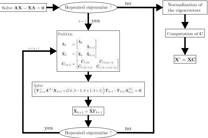
To determine an eigenvector matrix that is continuously differentiable, (4.10) has to be solved recursively. When repeated eigenvalues occur, (4.10) has to be evaluated for the first order derivative. If (some of) the eigenvalues of the resulting matrix are still the same, then (4.10) has to be evaluated once more for the second order derivative. This process has to be repeated until (4.10) does not result in any repeated eigenvalues. At each iteration step the eigenvectors have to be updated by multiplication of theΓmatrix. This iterative process is illustrated in Figure 4.1. After that all the blocks ofΓhave been determined, the only thing left is the normalization of the eigenvectors as in (3.3) taking (3.4) into account and computing the coefficient matrixC1.
After a continuously differentiable eigenvector matrix has been found, i.e., in factΓ, the coefficient matrix C1 can be determined. For this, the same recurrence relation as in the conjecture is used. Also these relations are a result of extending the procedure of the simple cases presented in the previous section,
C1,mn:=
1
m
λ(m−1)I−Λ(m−1)
m −1
Γ−m1 (4.14a)
×Y∗mA(m)Xn+L(m, m−1, m, n) ifm < n,
C1,mn:=
1
nΓ
−1
m
Y∗mA(n)Xn+L(m, m−1, m, n)
(4.14b)
×λ(n−1)I−Λ(nn−1)− 1
For the diagonal matrices C1,mm for m = 1, . . . , n+ 1, it holds that only the
off-diagonal entries can be determined by the following formula,
Λ(mm−1)C1,mm−C1,mmΛ(mm−1):=
(4.15)
1
mΓ
−1
m
Ym∗A(m)Xm−Λm(m)+L(m, m−1, m, m).
Finally, the diagonal entries ofC1can then be found by
(4.16) ckk=−
N
l=1
l=k xmlclk,
analogously as for the simple cases in the previous section. After the determination ofC1, the first order derivative of the eigenvector matrix X′ can be found.
The only thing that still has to be done is to findΛ′
1. IfΛ1still contains repeated eigenvalues, then the whole process described in this section has to be performed for Λ1 again. If Λ1 only consists of distinct eigenvalues, then Λ1 is computed by determining the diagonal ofY∗1A′X1, since
(4.17) Y∗1A′X1−Λ′1=−Λ1C1,11+C1,11Λ1.
[image:11.612.120.467.389.620.2]By comparing the diagonal entries on both left and right-hand side, the statement follows.
Finally, a last remark has to be given. The fact thatΛ1can still contain repeated eigenvalues ensures thatΓ1 does not have to be a diagonal matrix, but this matrix is unknown. However, the fact thatΓ commutes with Λ and that no higher order derivative ofΛ1 occurs,Γ1 disappears from (4.10), and therefore, definition (4.13) is justified.
5. Examples. In this section, the generalization of the method presented in the previous section will be illustrated by some examples. The first three examples show that the three simple cases discussed in Section 3 fit with the general algorithm. The fourth example is a numerical example.
Example 5.1. If all eigenvalues ofΛare distinct, then the only thing left for the
eigenvectors is to normalize them according to (3.3), taking (3.4) into account. To compute the coefficient matrix C1 and the eigenvalue derivative matrix Λ′, writing out (4.15) in coordinates form= 1 results in (3.1) and (3.2), but now the values of
γk fork= 1, . . . , N are already known from the normalization. The diagonal entries of C1 do not follow from (4.15), but from (4.16) which is identical to (3.5), where again allγk are known.
Example 5.2. If Λ contains a repeated eigenvalue, then a partitioning (4.6) has to be performed on Λ for n = 1 and a similar one on the eigenvector matrix
¯
X and coefficient matrix C. This partitioning is equal to (3.6). Next, (4.10) has to be evaluated for n = 1. In this case, matrix L is equal to zero, and therefore, (4.10) indeed reduces to (3.7d). Since this eigensystem does not yield any repeated eigenvalues again, also here the normalization of the eigenvectors takes place and the computation of C1 can be carried out by using (4.14b), (4.14a), (4.15) and (4.16) again.
Example 5.3. If bothΛ and the eigenvalues of system (3.7d) contain repeated
eigenvalues, then partitioning (4.6) has to be performed forn= 2. Similarly, parti-tioning (4.8) is applied to the eigenvector matrix ¯Xand coefficient matrix C. The result resembles the partitioning of (3.12). The evaluation of (4.10) returns the first nontrivial case, sinceL is nonzero, viz.
L(2,1,3,3) = 2Y3∗A′X1(λI−Λ1)−1Y1∗A′X3= 2 ¯Y∗3A′X¯1(λI−Λ1)−1Y¯∗1A′X¯3Γ3.
With this L, (4.10) reduces to (3.14). Because this eigensystem is assumed to have only distinct eigenvalues, we can proceed by normalizing the eigenvectors and com-putingC1in a similar way as in the previous simple case.
Example 5.4. This example illustrates the method given by Figure 4.1 for a
ma-trix of which we can compute the eigenvalues and eigenvectors analytically. Therefore, the results of the numerical method presented in this paper can be verified immedi-ately, because the derivatives of the eigenvalues and eigenvectors are also available analytically. LetAbe given by
A(p) := 1 2(1 +p2)
a11(p) a12(p) a13(p)
a21(p) a22(p) a23(p)
a31(p) a23(p) a33(p)
with
a11(p) = 2 cos(p)(−2+2p2+(1+p2) cos(2p)−4p2sin(p)),
a12(p) = 8p(−2 cos(p)+sin(2p)),
a13(p) = (−3+5p2) cos(p)−(1+p2) cos(3p)−4p2sin(2p),
a21(p) = 4p(−2 cos(p)+sin(2p)),
a22(p) =−2 cos(p)(−5+3p2+8 sin(p)),
a23(p) = 4p(−2 cos(p)+sin(2p)),
a31(p) = (−3+5p2) cos(p)−(1+p2) cos(3p)−4p2sin(2p),
a32(p) = 8p(−2 cos(p)+sin(2p)),
a33(p) = 2 cos(p)(−2+2p2+(1+p2) cos(2p)−4p2sin(p)).
The (analytical) eigenvalues are then
(5.1) λ1(p) = cos(3p), λ2(p) = 5 cos(p)−4 sin(2p), λ3(p) =−3 cos(p).
For p = π/2, we see that λ(1k) = λ (k)
2 = λ
(k)
3 for k = 0,1,2, and λ (k)
1 = λ
(k) 2 for
k= 0,1, . . . ,5. The eigenvectors can also be found analytically, and if normalization (3.4) atp=π/2 is used, then they are given by
(5.2) X=
−1 1 1/p
0 −1/p 1
1 1 1/p
.
In general, the analytical expressions for the eigenvalues and eigenvectors is hard, if not impossible to obtain. At p = π/2, A reduces to the identity matrix. Since any 3×3 matrix is a candidate for an eigenvector matrix, we just take the identity matrix. Because the analytical form of the eigenvector matrix is available, we already know that this choice of the eigenvector matrix is not continuously differentiable. To find a continuously differentiable eigenvector matrix, we use the algorithm illustrated in Figure 4.1. Note that in this example outcomes are given in 4 decimals.
Initialization step:
A=I3×3, Λ1=∅,Λ2=03×3,X1=∅,X¯2=I3×3. Step 2:
A′ = 3I3×3,Λ2=∅,Λ3= 3I3×3,X2=∅,X¯3=I3×3. Step 3:
A′′=03×3,Λ3=∅,Λ4=03×3,X3=∅,X¯4=I3×3. Step 4:
A(3)=
−23.5392 10.8724 3.4608 5.4362 −9.9216 5.4362 3.4608 10.8724 −23.5392
Λ4=−3,Λ5=−27I2×2,X4=
0.4731 0.7432 0.4731
,X¯5=
0.4187 −0.9541
−0.3938 0.2525 0.8183 0.1608
.
Step 5:
A(4)=
−12.5425 −11.7169 −12.5425
−5.8584 25.0849 −5.8584
−12.5425 −11.7169 −12.5425
,
Λ5=∅,Λ6=02×2,X5=∅,X¯6=
0.4187 −0.9541
−0.3938 0.2525 0.8183 0.1608
.
Step 6:
A(5)=
202.5537 −63.9949 −40.4463
−31.9975 −36.1074 −31.9975
−40.4463 −63.9949 202.5537
,
Λ6=
3.2283 0 0 243.0000
,X6=
−0.7161 0.5771 0.4559 0
−0.7161 −0.5771
.
Since no repeated eigenvalues occur anymore, the continuously differentiable eigenvector matrix has been determined up to the normalization. When the nor-malization (3.3) has been performed,Xequals
X=
1.0000 −1.0000 0.6366
−0.6366 0.0000 1.0000 1.0000 1.0000 0.6366
,
which, of course, is equal to the analytical solution ofXgiven in (5.2) forp=π/2. The next step is to determineC. Because several blocks in the partitioning ofΛ are empty,C only consists of the following blocks
C=
C44 C46 C64 C66
.
The blocks C46 and C64 and the off-diagonal entries of C66 can be determined by using (4.14a), (4.14b) and (4.15), respectively. The diagonal entries of C can be computed by using (4.16). As a consequence,Cequals
C=
−0.2884 −0.1836 0.0000 0.0000 0.0000 0.0000
−0.1836 0.2884 0.0000
To conclude this example, the eigenvalue and eigenvector derivative matrix are given by
Λ′=
Λ′4 Λ′6
=
3 0 0
0 3 0
0 0 3
,
X′=XC=
0.0000 0.0000 −0.4053 0.4053 0.0000 0.0000 0.0000 0.0000 −0.4053
.
Note that the outcome is of course equal to the analytical derivatives of the eigenvalues and eigenvectors as given by (5.1) and (5.2) after substitution ofp=π/2.
REFERENCES
[1] E. Andersonet al. LAPACK User’s Guide, 3rd edition. SIAM, Philadelphia, 1999.
[2] A.L. Andrew. Convergence of an iterative method for derivatives of eigensystems. Journal of Computational Physics, 26:107–112, 1978.
[3] A.L. Andrew and R.C.E. Tan. Computation of derivatives of repeated eigenvalues and the corresponding eigenvectors of symmetric matrix pencils. SIAM Journal on Matrix Analysis and Applications, 20:78–100, 1998.
[4] M.I. Friswell. The derivatives of repeated eigenvalues and their associated eigenvectors. Journal of Vibration and Acoustics, 118:390–397, 1996.
[5] W.C. Mills-Curran. Calculation of eigenvector derivatives for structures with repeated eigenval-ues. AIAA Journal, 26:867–871, 1988.
[6] M.G. Moharamet al. Stable implementation of the rigorous coupled-wave analysis for surface-relief gratings: enhanced transmittance matrix approach. Journal of the Optical Society of America A, 12:1077–1086, 1995.
[7] D.V. Murthy and R.T. Haftka. Derivatives of eigenvalues and eigenvectors of a general complex matrix.International Journal For Numerical Methods in Engineering, 26:293–311, 1988. [8] R.B. Nelson. Simplified calculation of eigenvector derivatives. AIAA Journal, 14:1201–1205,
1976.