Full Terms & Conditions of access and use can be found at
http://www.tandfonline.com/action/journalInformation?journalCode=ubes20
Download by: [Universitas Maritim Raja Ali Haji] Date: 13 January 2016, At: 00:30
Journal of Business & Economic Statistics
ISSN: 0735-0015 (Print) 1537-2707 (Online) Journal homepage: http://www.tandfonline.com/loi/ubes20
Duration Dependence in Stock Prices
Asger Lunde & Allan Timmermann
To cite this article: Asger Lunde & Allan Timmermann (2004) Duration Dependence in Stock Prices, Journal of Business & Economic Statistics, 22:3, 253-273, DOI: 10.1198/073500104000000136
To link to this article: http://dx.doi.org/10.1198/073500104000000136
Published online: 01 Jan 2012.
Submit your article to this journal
Article views: 187
View related articles
Duration Dependence in Stock Prices:
An Analysis of Bull and Bear Markets
Asger L
UNDEDepartment of Information Science, The Aarhus School of Business, Aarhus, Denmark (alunde@asb.dk)
Allan T
IMMERMANNDepartment of Economics, University of California, San Diego, La Jolla, CA 92093-0508 (atimmerm@ucsd.edu)
This article studies time series dependence in the direction of stock prices by modeling the (instantaneous) probability that a bull or bear market terminates as a function of its age and a set of underlying state variables, such as interest rates. A random walk model is rejected both for bull and bear markets. Although it ts the data better, a generalized autoregressive conditional heteroscedasticity model is also found to be inconsistent with the very long bull markets observed in the data. The strongest effect of increasing interest rates is found to be a lower bear market hazard rate and hence a higher likelihood of continued declines in stock prices.
KEY WORDS: Hazard model; Interest rate effect; Survival rate.
1. INTRODUCTION
Since the seminal work by Samuelson (1965) and Leroy (1973), the random walk and martingale models of stock prices have formed the cornerstone of modern nance. Hence it is not surprising that an extensive empirical literature has considered deviations from these benchmark models. Several authors, in-cluding Lo and MacKinlay (1988), Fama and French (1988), Poterba and Summers (1988), Richardson and Stock (1989), and Boudokh and Richardson (1994), have studied long-run se-rial correlations in stock returns. Although this literature re-ports indications of a slowly mean reverting component in stock prices, deviations from normally distributed returns, time-varying volatility, and small sample sizes have plagued exist-ing tests and made it difcult to conclusively reject the random walk model.
This article proposes a new approach to modeling time se-ries dependence in stock prices that allow bull and bear hazard rates—that is, the probability that a bull or bear market termi-nates in the next period—to depend on the age of the market. Inspection of these hazard rates yields new insights into long-run dependencies and deviations from parametric models of asset prices proposed in the literature, including the simple ran-dom walk model with a constant drift and models that allow for volatility persistence.
By explicitly focusing on duration dependence in stock prices, the proposed tests are very different from the tests based on autocorrelations previously adopted in the literature. The tests are more closely related to the duration dependence mea-sures rst proposed in the context of regime switching models used to analyze gross domestic product growth (Durland and McCurdy 1994) or stock market prices (Maheu and McCurdy 2000a). Although the two approaches share some of the same objectives—to capture potential duration dependence—they differ both in terms of the denition of the underlying states and in terms of econometric methodologies.
Our approach does not require that stock prices follow a low-order Markov process, although this is a special case of our model when termination probabilities are memoryless. Faust (1992) demonstrated that existing tests for autocorrela-tion based on variance ratios have optimal power in testing the
random walk hypothesisagainst certain classes of stationary au-toregressive moving average models. However, these models form only a small subset of the alternatives that are interest-ing from an economic standpoint, such as nonlinear speculative bubble processes and processes in which the drift depends on past cumulated returns within a state. There is no result for the power of autocorrelation tests against nonlinear alternatives or processes with long memory. This is important, because there is mounting evidence of nonlinearities such as a switching fac-tor in the mean and volatility of stock returns (cf. Maheu and McCurdy 2000a; Perez-Quiros and Timmermann 2000).
We formalize bull and bear states in terms of a lter that tracks movements between local peaks and troughs. Earlier studies, such as those of Fabozzi and Francis (1977), Kim and Zumwalt (1979), and Chen (1982), considered denitions of bull markets based simply on returns in a given month exceed-ing a certain threshold value. Fabozzi and Francis (1977) also considered a denition of bull markets based on “substantial” up-and-down movements. In this denition, a substantial move in stock prices occurs whenever the absolute value of stock re-turns in a given month exceeds half of one standard deviation of the return distribution. Such denitions do not reect long-run dependencies in stock prices, and they ignore information about trends in stock price levels. According to our denition, the stock market switches from a bull state to a bear state if stock prices have declined by a certain percentage since their previous (local) peak within that bull state. Likewise, a switch from a bear state to a bull state occurs if stock prices experience a similar percentage increase since their local minimum within that state. This denition does not rule out sequences of neg-ative (positive) price movements in stock prices during a bull (bear) market as long as their cumulative value does not exceed a certain threshold. By abstracting from the small unsystematic price movements that dominate time series as noisy as daily price changes, this denition is designed to capture long-run dependencies in the underlying drift in stock prices.
© 2004 American Statistical Association Journal of Business & Economic Statistics July 2004, Vol. 22, No. 3 DOI 10.1198/073500104000000136 253
We nd evidence of distinctly different duration dependence in bull and bear states. Controlling for interest rates, the longer a bull market has lasted, the lower its hazard rate and hence the lower the probability that it terminates in the next period. In contrast, in bear markets the hazard rate tends to be highest at long durations. Interest rates are also found to have an important effect on hazard rates. Increases in the interest rate are associ-ated with a small increase in the bull market hazard rate and with a large decrease in the bear hazard rate. They are therefore associated with a higher probability of being in a bear market and a lower probability of being in a bull market. The nding of a hazard function that depends on the age of the state suggests that stock prices do not follow a low-order Markov process. In-stead, the drift and the effect of interest rates on stock prices appear to be related to the market’s memory of the time spent in the current state. This means that the effect of an interest rate change on stock prices depends on the age and type of the state in which the change occurs.
Most closely related to the current study are the articles by Maheu and McCurdy (2000a) and Pagan and Sossounov (2000). Pagan and Sossounov (2000) also considered a den-ition of bull and bear states based on cumulative price changes; their study characterized movements in stock prices through the average duration and amplitude of bull and bear markets. The Pagan–Sossounov dating method is based on a modication of the Bry–Boschan algorithm and seeks out local peaks and troughs within a predetermined window of data points subject to a set of censoring rules that restrict both the minimum length of the bull/bear market (4 months) as well as the minimum du-ration of a full cycle (16 months) (see their app. B). Our lter does not use restrictions on the minimal length of the bull/bear states but requires choosing the value of the initial state and set-ting threshold values for the size of cumulative movements in stock prices that trigger a switch between these states.
Maheu and McCurdy (2000a) treated the state as an unob-served variable and classied monthly stock returns into two latent states based on a Markov switching model extended to account for duration-dependent state transitions. Whereas our regimes are dened according to the cumulative movements in stock prices and thus track local peaks and troughs in stock prices, their Markov-switching approach endogenously iden-ties a high-mean, low-variance bull state and a low-mean, high-variance bear state. This approach tends to identify turn-ing points more frequently than ours does. When the regime switching is restricted to only occur in the mean, in a “decou-pled” model, a state with a large negative mean return and a state with a small positive mean return are identied. Maheu and McCurdy (2000b) also studied a model in which regimes are present in the volatility but not in the mean. Whether an endogenous or an exogenous determination of the lter size is most appropriate depends, of course, on the purpose of the analysis.
The article is organized as follows. Section 2 presents our de-nition of bull and bear market states. Section 3 characterizes the unconditional distribution of the durations and returns in bull and bear markets using more than 100 years of daily stock prices from the United States. Section 4 considers a formal test for duration dependence, and Section 5 discusses estimation of bull and bear markets whose hazard rate may depend on the
age of the market. Section 6 reports empirical results and un-dertakes a scenario analysis to investigate the effect of an inter-est rate change on bull and bear hazard rates. Section 7 briey discusses further economic interpretations of our ndings.
2. DEFINITION OF BULL AND BEAR MARKETS
Financial analysts and stock market commentators frequently classify the underlying trend in stock prices into bull and bear markets. Durations of bull and bear markets are key compo-nents of the risk and return characteristics of stock returns, so understanding their determinants is clearly important. Yet de-spite this importance, little work has been done on formalizing these concepts and investigating whether bull and bear states provide a useful way of characterizing long-run dependencies in stock prices. It is not clear, for example, whether such states serve a purely descriptive purpose or whether the knowledge that stock prices have been in a particular state for a certain length of time affects the conditionaldistribution of future price movements. In the latter case, investment performance conceiv-ably could be improved by conditioning on the type and age of the current state.
There is no generally accepted formal denition of bull and bear markets in the nance literature. One of the few au-thors who have attempted to dene bull and bear markets is Sperandeo (1990), who dened bull and bear markets as fol-lows:
Bull market: A long-term: : :upward price movement characterized by a series of higher intermediate: : :highs interrupted by a series of higher intermediate lows.
Bear market: A long-term downtrend characterized by lower intermediate lows interrupted by lower intermediate highs (p. 102).
More recently, Chauvet and Potter (2000) offered a similar def-inition. To formalize the idea of a series of increasing highs in-terrupted by a series of higher intermediate lows, letItbe a bull market indicator variable taking the value 1 if the stock market is in a bull state at timet and 0 otherwise. Assume that time is measured on a discrete scale and that the stock price at the end of periodtisPt. Let¸1be a scalar dening the threshold of the movements in stock prices that trigger a switch from a bear to a bull market, and let¸2be the threshold for shifts from a bull to a bear market. Suppose that att0, the stock market is at a local maximum (It0D1) and setP
max
t0 DPt0, wherePt0 is
the value at timet0of the stochastic process tracking the stock price. Let¿maxand¿min be stopping-time variables dened by the conditions process crosses one of the two barriersfPmaxt
0 ,.1¡¸2/P
max t0 g. If ¿max< ¿min, then we update the local maximum in the current bull market state,
Pmaxt
0C¿max DPt0C¿max; (2)
Lunde and Timmermann: Duration Dependence in Stock Markets 255
then the bull market has switched to a bear market that prevailed fromt0C1 tot0C¿min:It0C1D ¢ ¢ ¢ DIt0C¿minD0. In this case,
we setPmint
0C¿min DPt0C¿min. If the starting point att0 is a bear
market state, then the stopping times are dened as
¿min
This denition of bull and bear states partitions the data on stock prices into mutually exclusive and exhaustive bull and bear market subsets based on the sequences of rst passage times. The resulting indicator function,It, gives rise to a random variable,T, that measures the durations of bull or bear markets. These are given simply as the time between successive switches inIt.
We consider a range of values for¸1 and¸2. The smaller the values at which these parameters are set, the more bull and bear market spells we expect to see. This is likely to improve the power of our statistical tests as the sample size used in the duration analysis increases. However, there are also limits to how low¸1 and ¸2 can be set because too-small values will lead our analysis to capture short-term dynamics in stock price movements. A value of¸2D:20 is conventionally used in the nancial press, so we entertain this along with smaller values. Setting¸1> ¸2provides a way to account for the upward drift in stock prices, which works against nding many bear mar-kets. We consider four lters.¸1; ¸2/, expressed in percentage terms:.20;15/,.20;10/,.15;15/, and .15;10/. The .15;15/ parameterization allows us to study the effect of using a sym-metric lter.
The focus on local peaks and troughs allows us to concen-trate on the systematic up-and-down movements in stock prices and to lter out short-term noise. This is an important consid-eration for data as noisy as daily stock price changes. Although some arguments can be made in favor of imposing an additional minimum duration constraint, this also adds an extra layer of complexity and means that the data must be ltered through a recursive pattern recognition algorithm, as explained by Pagan and Sossounov (2000). Instead, our approach models both short and long durations, but allows the hazard rate to differ across durations.
Naturally, our lter is related to a wide literature on techni-cal trading rules that models lotechni-cal trends in stock prices (cf. Brock, Lakonishok, and Lebaron 1992; Brown, Goetzmann, and Kumar 1998; Sullivan, Timmermann, and White 1999). However, the similarities between technical trading rules and duration measures are only supercial. Technical trading rules search for patterns in prices conditional on a time horizon that is typically quite short. For example, the value of a 100-day moving average of prices may be compared with the value of a 25-day moving average. In contrast, we do not condition on
the time of a particular movement, but instead explicitly treat this as a random variable whose distribution we are interested in modeling.
3. DURATIONS OF BULL AND BEAR MARKETS
3.1 Data
To investigate the properties of bull and bear market states us-ing the denition proposed in Section 2, we construct a dataset of daily stock prices in the United States from 2/17/1885 to 12/31/1997. From 2/17/1885 to 2/7/1962, the nominal stock price index is based on the daily returns provided by Schwert (1990). These returns include dividends. From 3/7/1962 to 12/31/1997, the price index is constructed from daily returns on the Standard & Poor 500 (S&P500) price index, again in-cluding dividends and obtained from the CRSP tapes. Combin-ing these series generates a time series of 31,412 daily nominal stock prices.
Ination has varied considerably over the sample period, and it can be argued that the drift in nominal prices does not have the same interpretation during periods of low ination and high in-ation. To deal with effects arising from this, we consider both nominal and real stock prices. To construct real stock prices, we build a daily ination index as follows. We use monthly data on the consumer price index (from Shiller 2000) and con-vert it into daily ination rates by solving for the daily ina-tion rate such that the daily price index grows smoothly—and at the same rate—between subsequent values of the monthly con-sumer price index. Finally, we divide the nominal stock price index by the consumer price index to get a daily index for real stock prices. Because the volatility of daily ination rates is likely to be only a fraction of that of daily stock returns, nor-malizing by the ination rate has the effect of a time-varying drift adjustment. Lack of access to daily ination data is un-likely to affect our results in any important way.
We also consider the effect of time-varying interest rates on hazard rates. Because there is no continuous data series on daily interest rates from 1885 to 1997, we construct our data from four separate sources. For data from 1885 to 1889, the source is again Shiller (1989). For data from 1890 to 1925, we use the interest rate on 90-day stock exchange time loans as reported in Banking and Monetary Statistics(Board of Governors, Federal Reserve System 1943). These rates are provided on a monthly basis, and we convert them into a daily series by simply apply-ing the interest rate reported for a given month to each day of that month. For data from 1926 to 1954, we use the 1-month Treasury Bill rates from the risk-free rates le on the CRSP tapes, again reported on a monthly basis and converted into a daily series. Finally, for data from July 1954 to 1997, we use the daily Federal Funds rate. These three sets of interest rates are concatenated to form one time series covering the full sample. We consider nominal interest rates in the analysis of nominal stock prices and real interest rates—computed as the difference between the daily interest and ination rate—in the analysis of real stock prices.
Much of standard survival analysis in economics and nance assumes continuouslymeasured data. But, because we use daily data and do not follow price movements continuously,our data
are interval censored, and the termination of our durations is known to lie only between consecutive follow-ups. Effectively, the measurement ofT, the duration of bull and bear markets, is divided intoAintervals,
[a0;a1/;[a1;a2/; : : : ;[aq¡1;aq/;[aq;1/; whereqDA¡1 and only the discrete time durationT2 f1; : : : ;Agis observed, whereTDtdenotes termination within the interval [at¡1;at/. Although we draw on approaches from the literature on eco-nomic duration data (see, e.g., Kiefer 1988; Kalbeisch and Prentice 1980; Lancaster 1990), this also means that we must be careful when modifying the standard tools from continuous time analysis.
3.2 Random Walk Model
The natural benchmark that has underpinned much of the analysis in nancial economics is the random walk model. This model, which has also been considered by Pagan and Sossounov (2000), assumes constant mean and volatility of stock price changes. To capture the duration distribution gen-erated by the random walk model, we simulate 2,000 samples of 31,412 daily price observations from this model. Both the drift and the volatility parameters were estimated to match the real or nominal stock price data.
Although simple, the random walk model has been surpris-ingly difcult to reject in many statistical tests, and it is also quite exible in tting bull and bear durations (cf. Pagan and Sossounov 2000). For example, it is able to generate longer bull market durations than bear durations simply by introducing a positive drift parameter.
3.3 Volatility Clustering
In many regards, the pure random walk model for stock prices is too simple. Most notably, the volatility of daily stock price changes is strongly serially correlated, which undoubt-edly will affect the duration distribution of our data. We are interested in documenting possible time series dependencies in the drift of stock prices, but also want to account for the ef-fects of time-varying conditional volatility. To accomplish this while accounting for both short-run and long-run persistence in volatility, we estimate the following generalized autoregres-sive condotional heteroscedasticity (GARCH) model proposed by Engle and Lee (1999) and extended to include an ARCH-in-mean effect:
rtD¹C¯rt¡1C° ¾tC"t; "t»N.0; ¾t2/;
¾t2DqtC®."t2¡1¡qt¡1/C¯.¾t2¡1¡qt¡1/; (5) qtD!C½.qt¡1¡!/CÁ."2t¡1¡¾t2¡1/:
We then compare the duration distribution of bull and bear mar-ket spells generated by this model to the duration distribution from the actual data. Again we simulate 2,000 samples each with 31,412 observations. Comparing the duration distribution under the random walk model with that under the GARCH model provides a way to account for the effect of volatility clus-tering.
3.4 Bull and Bear Durations
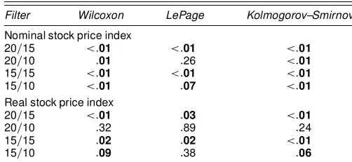
Insight into how our denition partitions stock prices into bull and bear spells is provided by Figure 1, which uses the real and nominal price indices to show the sequence of consecutive bull and bear markets over the full sample period 1885–1997. To better illustrate the individual episodes, we plot the natural logarithm of the real and nominal stock price index in eight separate windows. The gure uses a 20/10 lter that splits the sample into 66 bull and bear markets. Many of the bull mar-kets are very long, with the longest lasting from 1990 to 1997. Most of the short durations occur from 1929 to 1934, around the time of the Great Depression. For this period, the number of turning points identied by our method exceeds that found by Pagan and Sossounov (2000). This is a result of the increased stock market volatility during this period in conjunction with our turning point method, which does not impose a minimum length on each state.
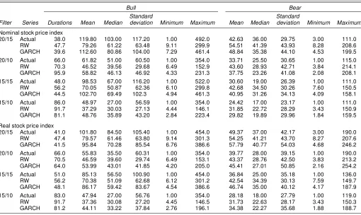
Table 1 presents descriptive statistics for the distribution of bull and bear market durations. Properties of bull and bear mar-ket states are reported in weeks, although it should be recalled that our analysis was carried out using daily data. We report re-sults for the four lter sizes.¸1; ¸2/described in the previous section. As the lter size declines, the means of the bull and bear durations decline, as do their standard deviations. Since lower thresholds will be crossed more frequently, this is to be expected and this effect is also observed in the data gener-ated by the random walk and GARCH models. Using nominal prices, the mean bull market duration is between two and three times as long as the mean bear duration, suggesting that be-tween two-thirds and three-quarters of the time is spent in the bull state. This proportion declines somewhat once we use real stock prices, which have a smaller positive drift. For real stock prices, the mean bull market duration exceeds the mean bear market duration by a factor of 1.5–2.3, depending on the lter size.
The standard deviation of the bull market durations observed in the actual data is systematically greater than that generated by the random walk and GARCH models. Conversely, the stan-dard deviation of the bear market durations in the actual data is lower than that produced by the benchmark models. This is reected in the much larger (smaller) values of the maximum duration for the actual bull (bear) market sample than in the simulated data. Though by no means formally proving that the benchmark models are unable to match the duration distribution observed for the actual data, these observations nevertheless in-dicate that the longest bull markets last too long, and the longest bear markets last too short to be compatible with our benchmark models.
The random walk model with a nonzero drift can capture some features of bull and bear markets, such as the asymme-try between bull and bear durations when a symmetric 15/15 lter is used. However, consistent with the ndings of Pagan and Sossounov (2000), this model also has clear shortcomings that are at odds with the data. Most notably, it cannot capture the behavior of the longest bull markets, or the shortest bear markets, such as those occurring in the late 1920s.
An alternative view of bull and bear market durations is pro-vided in Figure 2, which for the four lters plots the estimated
Lu
nd
e
a
nd
Ti
mm
er
m
an
n:
Durati
on
Dep
en
de
nc
e
in
Sto
ck
Ma
rke
ts
25
7
Figure 1. Bull and Bear Markets Based on the Nominal/Real S&P500 Stock Price Index (on log-scale) Using a 20/10 Filter. The fat line shows the real price index and the bottom shadings track the bull markets derived from this index, the thin line shows the nominal price index, and the top shadings track the bull markets derived from this index.
Table 1. Summary Statistics for Bull and Bear Market Durations
Bull Bear
Standard Standard
Filter Series Durations Mean Median deviation Minimum Maximum Mean Median deviation Minimum Maximum
Nominal stock price index
20/15 Actual 38.0 119:80 103:00 117:20 1.00 492.0 42.63 36.00 29.75 3.00 111.0 RW 47.7 79:26 61:22 63:48 9.11 299.9 54.51 41.39 43.93 8.28 208.6 GARCH 39.6 112:60 80:86 104:00 7.29 461.4 48.84 35.38 44.10 4.53 199.5 20/10 Actual 66.0 61:82 51:00 60:50 1.00 354.0 33.71 25.50 30.65 1.00 115.0 RW 70.3 46:52 39:56 29:68 6.49 152.9 43.60 28.93 42.71 3.84 214.1 GARCH 95.9 58:82 46:13 46:92 4.33 231.3 37.75 23.26 41.08 2.08 208.1 15/15 Actual 48.0 98:53 67:00 116:20 1.00 522.0 30.60 19.00 26.39 1.00 111.0 RW 56.2 70:05 50:87 62:36 6.10 299.8 42.68 34.50 30.26 7.60 150.5 GARCH 44.5 102:70 69:49 102:3 4.94 461.3 40.95 31.26 34.13 4.09 158.1 15/10 Actual 86.0 48:97 27:00 56:59 1.00 354.0 24.42 17.00 23.17 1.00 111.0 RW 91.7 37:29 30:03 27:13 4.44 146.1 31.85 22.72 28.29 3.43 150.9 GARCH 81.1 48:76 35:89 43:20 2.84 223.4 29.82 19.89 29.96 1.84 159.5
Real stock price index
20/15 Actual 41.0 101:80 84:50 105:40 1.00 454.0 49.37 37.00 42.17 3.00 190.0 RW 47.4 79:57 61:46 63:80 9.14 301.3 54.25 41.21 43.70 8.27 207.6 GARCH 41.5 95:84 70:28 85:54 6.76 386.6 57.79 40.77 54.03 4.68 246.2 20/10 Actual 66.0 55:83 35:50 60:31 1.00 354.0 39.77 28.00 39.15 1.00 190.0 RW 70.5 46:59 39:60 29:74 6.49 153.1 43.37 28.76 42.50 3.83 213.2 GARCH 64.0 53:99 43:01 41:85 4.20 205.0 45.41 27.01 50.85 2.16 254.2 15/15 Actual 51.0 85:13 56:50 100:90 1.00 454.0 36.84 25.00 35.18 1.00 136.0 RW 56.2 70:38 51:09 62:68 6.12 301.2 42.54 34.39 30.13 7.59 149.7 GARCH 48.1 86:17 59:42 83:67 4.54 386.6 46.74 35.00 40.12 4.17 187.9 15/10 Actual 83.0 47:94 27:00 56:76 1.00 354.0 28.18 18.00 27.79 1.00 119.0 RW 91.7 37:36 30:08 27:20 4.45 146.5 31.73 22.63 28.17 3.43 150.3 GARCH 81.2 44:11 33:22 37:84 2.76 196.1 34.38 22.27 35.68 1.88 188.7
NOTE: The simulated durations are generated from 2,000 random walk (RW) or GARCH series, each with 31,412 observations.
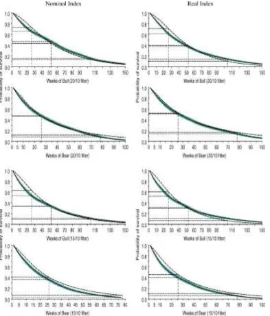
densities of bull and bear market durations using a Gaussian kernel smoother. The rst two rows show results for nominal stock prices, and the last two rows are based on real prices. Also ploted are the densities for the simulated random walk and GARCH models. Major differences in the duration den-sities of bull and bear markets are seen relative to what would be expected under the benchmark models, even after adjusting for time-varying volatility as is done in the GARCH model. The bull market density is lower at short durations and higher at long durations compared with the simulated models. In contrast, at short durations the bear duration density is generally higher in the actual data than in the simulations. Notice how GARCH ef-fects generally lead to a higher probability of very short bull or bear markets compared with the random walk model. This is consistent with the intuition that volatility effects are strongest at high frequencies.
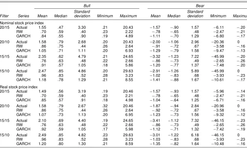
To show how much returns vary across bull and bear states, Table 2 reports return statistics for these states. Depending on the lter size, mean returns vary from 1.5% to 2.5% per week in bull markets and from¡3:4% to ¡1:5% percent per week in bear markets. These gures are computed as the mean return per bull or bear market converted into a weekly number. The unconditionalreal stock return of 6% per year can be computed as the duration-weighted average return per bull or bear market spell.
A larger asymmetry shows up in the median returns, which are generally 50–100% larger in absolute terms for bear than for bull markets. Although bear markets are much shorter than bull markets, the downward drift in bear markets is thus stronger than the upward drift in bull markets. Interestingly, the extent of
this asymmetry is not captured by the random walk or GARCH models, which are far closer to symmetry in median returns.
4. STATISTICAL TESTS OF DIFFERENCES IN DURATION DISTRIBUTIONS
So far we have uncovered a number of disparities between the duration distribution observed in the actual data and that generated by the simulated benchmark models, but we have not formally tested whether the two sets of duration distributionsre-ally differ. In this section we apply a battery of tests to compare the distributional properties of the data against those produced by the benchmark models.
Because there is no closed-form distribution for any of the duration models, we apply nonparametric two-sample tests to compare the actual and simulated data. (Detailed descriptions of these tests have been given by Hollander and Wolfe 1999.) In all cases we haveNDmCnduration spellsx1; : : : ;xm and y1; : : : ;yn from the two distributions. Under the null, it is as-sumed that thex’s andy’s are mutually independent draws from continuous distribution functionsFandG. To test for equality of the mean duration, we rst apply the Wilcoxon, Mann, and Whitney test,
H0:E.X/¡E.Y/D0:
The test is computed by ordering the combined sample of dura-tions in ascending order. Denote the rank ofyiin the joint order-ing bysiforiD1; : : : ;n, and let the rank sum of theYvalues
Lu
nd
e
a
nd
Ti
mm
er
m
an
n:
Durati
on
Dep
en
de
nc
e
in
Sto
ck
Ma
rke
ts
25
9
Figure 2. Kernel-Smoothed Densities of Bull and Bear Market Durations Derived From Different Filters. The simulated durations are generated from 2,000 random walk or GARCH series each with 31,412 observations (— actual data;¢¢¢¢¢GARCH; - - - random walk).
Table 2. Summary Statistics for Bull and Bear Market Returns
Bull Bear
Standard Standard
Filter Series Mean Median deviation Minimum Maximum Mean Median deviation Minimum Maximum
Nominal stock price index
NOTE: The simulated durations are generated from 2,000 random walk (RW) or GARCH series, each with 31,412 observations.
be dened asWDPnjD1sj. For test purposes, we use the stan-dardized version ofW,
W¤DWp¡E0.W/
To test for differences in either the dispersion or the location of the two duration distributions, we adopt the Lepage test. This test establishes whether there are differences in either the loca-tion parametersµ1andµ2or the scale parameters´1and´2of the two distributions. The null hypothesis is
H0:µ1Dµ2and´1D´2:
To compute the test, suppose that a score of 1 is assigned to both the smallest and the largest observations in the combined sample, a score of 2 is assigned to both the second-smallest and the second-largest observations, and so forth. The resulting score sum of observations drawn from theY sample, denoted byRj, is given byCDPnjD1Rj. This can be normalized to give
The Lepage test statistic is simply the sum of the squares ofW¤andC¤,
DD.W¤/2C.C¤/2»aÂ22: (7) Finally, to test for general differences in the two populations, we adopt the Kolmogorov–Smirnov test, whose null hypothesis is that the two duration distributions are identical,
H0:F.t/DG.t/;
for everyt. The alternative hypothesis is that the two duration distributions differ, that is,F.t/6DG.t/. The resulting test
Lunde and Timmermann: Duration Dependence in Stock Markets 261
(Critical values of the sample distribution have been given in, e.g., Hollander and Wolfe 1999.)
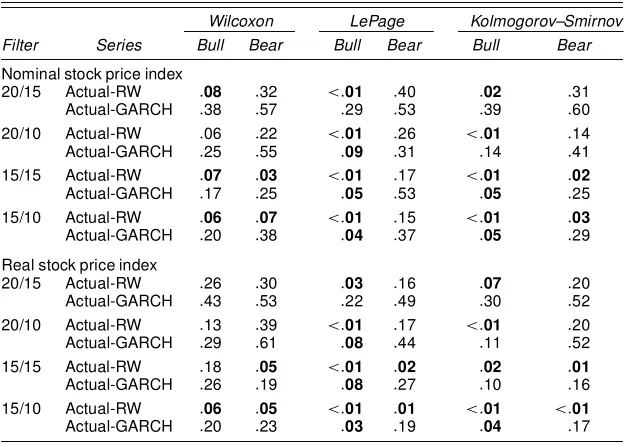
4.1 Empirical Findings
The outcome of these tests is reported in Table 3. In bull markets there is very strong evidence against the random walk model which is rejected at the 10% level by all tests based on nominal stock prices. This model also gets rejected by the LePage and Kolmogorov–Smirnov tests in the case of real stock prices. In the bear state the evidence is insufciently strong to lead to a rejection of the random walk model for the larger l-ters (20/15 and 20/10), but this model is generally rejected when the smaller lters (15/15 and 15/10) are used. This difference is most likely related to the power of the duration tests, because the smaller lters generate more duration spells than the larger ones (cf. Table 1).
Although it is more difcult to reject the null of equality of the duration distributions generated by the GARCH model and the actual data, in bull markets the null is nevertheless rejected by the LePage and Kolmogorov–Smirnov tests using the small lter sizes. In bear markets the null is not rejected at the 10% level. Failure to reject the null hypothesis for bear markets is again likely at least partially to reect low power. Indeed, as the lter size declines and the tests become more powerful, the pvalues decline from around .50 to around .20.
These results suggest that the Lepage and Kolmogorov– Smirnov tests produce signicant evidence against the two parametric models, particularly for the smaller lter sizes. The random walk model clearly cannot match the duration distribu-tion of either bull or bear markets. Although the GARCH model does a better job at tting the data, it still does not fully capture the properties of bull market durations. Because the LePage and Kolmogorov–Smirnov tests have power against differences in the dispersion of the duration distributions, our results suggest that these tests pick up differences related to the very long bull markets observed in the data.
5. MODELS OF DURATION DEPENDENCE IN BULL AND BEAR MARKETS
Section 3 characterized the unconditionaldistribution of bull and bear market spells. However, if the age of a bull or bear market affects future price movements then investors will want to calculate expectations conditional on the path followed by stock prices up to a given point in time. For instance, during the long bull market of the 1990s, concern was often expressed that this bull market was at greater risk of coming to an end because it had lasted “too long” by historical standards. This indicates a belief that the bull market hazard rate depends positively on its duration. The opposite view is that bull markets gain momen-tum; the longer a bull market has lasted, the more robust it is, and hence the lower its hazard rate.
Testing these hypotheses requires that we go well beyond inspecting the unconditional probability of termination for the bull or bear markets. Instead, the duration data must be char-acterized in terms of the conditional probability that the bull or bear state ends in a short time interval after some periodt, given that the state lasted up tot. For theith duration,Ti;this is measured by the discrete hazard function
¸i.tjXit/DPr.TiDtjTi¸t;Xit/; tD1; : : : ;A; (9) which is the conditional probability of termination in the in-terval [at¡1;at/given that this interval was reached in the rst place.XitD fxi1; : : : ;xitgis a vector of additional conditioning information, which will depend on the particular duration. Hy-potheses about the probability that a bull or bear market is ter-minated as a function of its age are naturally expressed in terms of the shape of this hazard function. For example, the natural null hypothesis is that the duration of the current state does not affect the hazard rate.
The probability that a bull or bear market lasts for a cer-tain time period can still be derived from these hazard rates. This is given as the discrete survivor function, which measures
Table 3. Two-Sample Tests for Equality of Duration Distributions
Wilcoxon LePage Kolmogorov–Smirnov Filter Series Bull Bear Bull Bear Bull Bear
Nominal stock price index
20/15 Actual-RW :08 :32 <:01 :40 :02 :31 Actual-GARCH :38 :57 :29 :53 :39 :60 20/10 Actual-RW :06 :22 <:01 :26 <:01 :14 Actual-GARCH :25 :55 :09 :31 :14 :41 15/15 Actual-RW :07 :03 <:01 :17 <:01 :02
Actual-GARCH :17 :25 :05 :53 :05 :25 15/10 Actual-RW :06 :07 <:01 :15 <:01 :03
Actual-GARCH :20 :38 :04 :37 :05 :29 Real stock price index
20/15 Actual-RW :26 :30 :03 :16 :07 :20 Actual-GARCH :43 :53 :22 :49 :30 :52 20/10 Actual-RW :13 :39 <:01 :17 <:01 :20 Actual-GARCH :29 :61 :08 :44 :11 :52 15/15 Actual-RW :18 :05 <:01 :02 :02 :01
Actual-GARCH :26 :19 :08 :27 :10 :16 15/10 Actual-RW :06 :05 <:01 :01 <:01 <:01
Actual-GARCH :20 :23 :03 :19 :04 :17
NOTE: This table reportspvalues from two-sample tests comparing the actual bull/bear market durations to those generated under the simulated random walk (RW) or GARCH models. The simulated durations are generated from 2,000 series, each with 31,412 observations.pvalues <.1 are highlighted in boldface.
the probability that a bull or bear market survives on the
inter-Common choices of hazard models are the probit, logit, and double exponential links (see Sueyoshi 1995 for such link func-tions). Throughout this article we use a logit link, that is,
¸i.tjXit/DF.x0it¯/D
exp.x0it¯ /
1Cexp.x0it¯ /: (11) We consider two separate models for these hazard rates. The rst model is a static model that assumes that the underlying parameters linking the covariates or state variables to the haz-ard rate do not vary over time and that the covariates are xed from the point of entry into a state. This makes our results di-rectly comparable with the large literature on univariate dynam-ics in stock prices surveyed by Campbell, Lo, and MacKinlay (1997, chap. 2). Under this assumption, the data take the form
fti;xiIiD1; : : : ;ng; where ti is the survival time and xi is a covariate (or state variable) observed at the beginning of the interval [ati¡1;ati/.
But switches between bull and bear market states are likely to be caused by changes in the underlying economic environment. For example, the drift in stock prices may turn from positive to negative as a result of increased interest rates or worsening eco-nomic prospects. The effect of such covariates may well depend on the age of the current bull or bear market. To account for this possibility, our second model extends the setup and allowsxit to be a vector that incorporates time-varying covariates. Now the data for theith duration spell takes the form
©
Because our data are discretely measured, the covariates follow a step function with jumps at the follow-up times,at. Within the interval [at¡1;at/, the history of covariates,
XitD.xi1;xi2; : : : ;xit/; is allowed to inuence the hazard rate¸i.tjXit/.
To allow for the possibility that the effect on the hazard rate of these covariates could depend on the age of the current state, we consider an approach that allows the parameters to vary with duration,
¸i.tjXit/DF.x0it®t/: (12)
The vector®tD.°0t;°0t/0comprises both the baseline and the covariance parameters. We use the rst-order random walk as our choice of transition equation determining the evolution in®t: tribution. This random walk specication has the advantage of not imposing mean reversion on the parameters, which are al-lowed to differ across durations (although neighboring points cannot be too far from each other) if the data support such vari-ation.
5.1 Estimation
The log-likelihood function can be conveniently set up using notation from the literature on discrete choice models. Consider the following discrete indicator variable:
yisD Using this notation, the contribution to the likelihood function from theith observation is
L i/
Thus, every spell the bull or bear market lives through con-tributes to the likelihood with the survivor probability 1¡¸i.sjxi/. Summing across duration spells, the total
log-An approach of treating the covariate parameters as xed ef-fects is appropriate only if the number of intervals is very small. In applications such as ours without enough intervals to apply continuous-time techniques, maximum likelihood estimates of a large number of parameters in the hazard functions of an un-restricted hazard model can be expected to have very poor sam-pling properties.
To get around this problem, we follow Fahrmeir (1994) and adopt state-space techniques that treat the hazard function as the measurement equation. Because our measurement equa-tion is nonnormal, it is complicated to solve for the poste-rior density of the hazard function conditional on the data, p.®1; : : : ;®qjy1; : : : ;yq;x1; : : : ;xq/, which is required for writ-ing down the likelihood function. We adopt the strategy, ad-vocated by Fahrmeir (1992), of basing estimation on posterior modes subject to smoothing priors that penalize large changes in neighboring parameters,®t¡®t¡1. As detailed in Appen-dix A, repeatedly applying Bayes’s theorem to the posterior
Lunde and Timmermann: Duration Dependence in Stock Markets 263
density, estimation of ®t by posterior modes is equivalent to maximizing the penalized log-likelihood function
lnL .®1; : : : ;®q/
D
n
X
iD1 ti
X
tD1
lit.®t/¡ 1
2.®0¡a0/ 0Q¡1
0 .®0¡a0/
¡1
2 q
X
tD1
.®t¡®t¡1/0Q¡1.®t¡®t¡1/; (17) where
lit.®t/Dyitln.F.x0it®t//C.1¡yit/ln
¡
1¡F.x0it®t/
¢
(18)
is the log-likelihood contribution of theith duration spell. The rst term measures the goodness of t of the model. The
sec-ond and third terms—which are introduced by the smoothness priors,Q0andQ, specied by the transition model—penalize large deviations between successive parameters and lead to smoothed estimates. Appendix B provides details on the numer-ical optimization of this penalized likelihood function through a generalized extended Kalman lter and smoother.
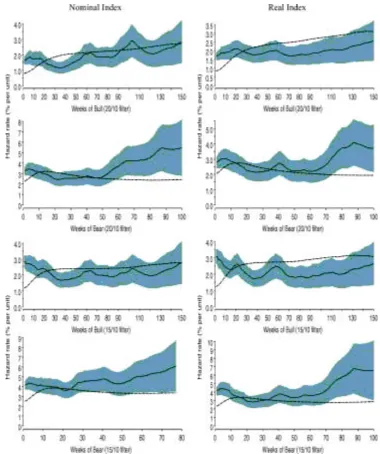
6. EMPIRICAL RESULTS
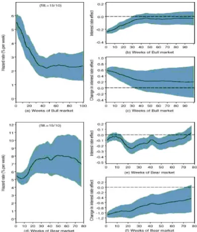
Using the estimation techniques and hazard models from Section 5, we rst estimate the hazard function for bull and bear markets in a model without time-varying covariates. The output from this exercise is the baseline hazard rates plotted in Figure 3 using lter sizes of 20=10 and 15=10. These baseline hazard rates measure the pure age dependence in bull and bear
Figure 3. Unconditional Hazard Rates for Bull and Bear Market Durations Derived From the Nominal and Real Stock Price Index and From 2,000 GARCH Series, Each With 31,412 Observations. Plots on the left are based on the nominal price index while the right plots are derived from the real price index. In all cases the hazard rate model assumes a logit link function:¸(t|Xi(t)) DF(xit0®t), wherexit0D1and®tD°0t,°0tD°0t¡1C»0t,
»0t» N(0,¾12), and°00» N(g0,¾02). The shaded area is 90% condence region (— actual; - - - simulated).
market termination probabilities. The panels on the left show the hazard rate estimated for the nominal price index, whereas the panels on the right plot estimates for real stock prices, in both cases surrounded by 90% condence regions. To establish a benchmark, we also plot the hazard rate under the GARCH model. Because it takes some time before the market moves the full distance of the lter, the hazard rate is initially very low un-der the GARCH model, but rapidly increases to a level of 2–4%. Once the initial threshold effect wears off, the GARCH hazard rates atten out.
These baseline hazard rates are surrounded by considerable estimation uncertainty, particularly at the long end, where the 90% condence intervals are very wide. Even so, some patterns emerge from these plots. First, the bear market hazard rates in-crease systematically at long durations, whereas the bull market hazard rates follow no particular pattern. This is another way of determining why long bear markets do not occur in the actual data, simply because of the rapid rise in bear hazard rates as their duration grows.
At short durations in the bull market, the simulated GARCH hazard rates are distinctly below the hazard rates observed in the actual data. This pattern is reversed at longer durations, where the GARCH hazard rates are higher than the actual hazard rates, at least for real stock prices. In bear markets the GARCH hazard rate is below its value in the actual data at both short and long durations, irrespective of whether nominal or real stock prices are considered. This is consistent with our earlier observation that the longest bull market durations are longer than what we expect from the parametric models, whereas the longest bear spells are shorter than what is consistent with these models.
To formally test whether the duration distribution for the bull and bear market states are identical, we adopted the two-sample tests from Section 4 to the bull and bear durations observed in the actual data. Irrespective of which test we use, Table 4 shows that we generally reject that bull and bear durations are drawn from the same distribution. This might be expected given the upward drift in both real and nominal stock prices, but this is by no means the only explanation for our ndings. For example, when the lter sizes are set so as to account for this drift (e.g., by using the 20/15 lter), the null of equality of the bull and bear duration distributions is strongly rejected by the actual data but not by the simulated data under the random walk model.
To provide a single summary measure of the attrition rates in bull and bear markets, Figure 4 plots the survivor function (10) for bull and bear states against the survival function under the
Table 4. Two-Sample Tests for Equality of Bull and Bear Durations
NOTE: pvalues below < .1 are highlighted in boldface.
simulated GARCH model. Again the left column is based on nominal prices and the right column is based on real prices. Although the individual hazard rates are estimated with con-siderable noise, the cumulated effects of differences in hazard rates at short and long durations becomes much clearer in this gure. In the bull market the survival probability at short du-rations is much lower in the actual data than in the simulated data. This changes at longer durations where the survival prob-ability becomes higher in the actual data than in the simulated data, particularly for real stock prices, where the 95% con-dence region lies entirely above the GARCH survivor function. A very different picture emerges in the bear state, where the survival function based on the actual data is always at or below that from the simulated data. For the smaller 15/10 lter, the full 95% condence region lies below the GARCH survival curve.
6.1 Interest Rate Effects
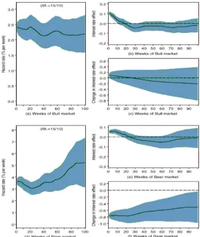
To shed light on how the hazard rates depend on the under-lying state of the economy, we next include interest rates as a time-varying covariate. Interest rates have been widely docu-mented to closely track the state of the business cycle and ap-pear to be a key determinant of stock returns at the monthly horizon (see, e.g., Kandel and Stambaugh 1990; Fama and French 1989; Glosten, Jagannathan, and Runkle 1993; Pesaran and Timmermann 1995; Whitelaw 1994). Interest ratelevels,it, may be affected by a low-frequency component and therefore might not contain the same information over a sample as long as ours, whereas interest ratechanges,1it, are more likely to track business cycle variation across the full sample. For this reason, we include both levels and changes in interest rates, so the set of covariates isx0itD.1;it; 1it/. Our analysis of nominal stock prices uses nominal interest rates, whereas our analysis of real stock prices is based on real interest rates. Our hazard spec-ication, which allows interest rate effects to vary with the age of the current state, is
¸i.tjxi.t//DF.°0tC°1titC°2t1it/: (19) Figure 5 shows the sequence of baseline hazards and nominal interest rate effects using nominal stock prices and a 15=10 l-ter. Compared with Figure 3, it is clear that controlling for inter-est rates has a signicant effect on the shape of the bull market baseline hazard. Controlling for interest rate effects, the market baseline hazard drops sharply from 5% to 2% per week as the bull market duration extends beyond 6 months. It remains at at longer durations. Young bull markets thus appear substantially more at risk of termination than bull markets that have lasted for 6 months or longer.
Figure 5(b) shows that at very short durations, higher nomi-nal interest rates are associated with a lower bull market hazard rate. However, this parameter is within one standard error of 0 after 30 weeks. The initial negative sign should be interpreted with caution, because interest rates tend to be high toward the beginning of a new expansion state, and this is often the begin-ning of a bull market in stock prices. More importanty, perhaps, positive interest rate changes are associated with increases in the bull hazard rate that are much larger in magnitude than the effects from the interest rate level [cf. Fig. 5(c)].
The baseline hazard in the bear market also changes as a re-sult of controlling for interest rate effects. The baseline hazard
Lunde and Timmermann: Duration Dependence in Stock Markets 265
Figure 4. Survivor Functions for Bull and Bear Markets Estimated From the Unconditional Hazard Rates Shown in Figure 3. Plots on the left are based on the nominal stock price index; plots on the right are derived from the real stock price index (— actual; - - - simulated; 95% condence bands).
rate now increases from 5% to about 8% per week at durations longer than 6 months. Both the interest rate level and interest rate changes are associated with negative effects on bear hazard rates that are more than one standard error away from 0 in most cases. Notice in particular the very large negative effect of in-terest rate increases on hazard rates in young bear markets. An environment of high and increasing interest rates thus leads to lower bear market hazard rates, which means a greater likeli-hood of remaining in the bear state.
Figure 6 illustrates results for the real stock price index. The baseline hazard rate declines in the bull market and increases after an initial slight decline in the bear state. The real interest rate level has a small positive correlation with both bull and bear hazard rates for durations up to 20 weeks and becomes nega-tive thereafter. Although real interest rate changes are
insignif-icantly correlated with hazard rates in the bull market, they are strongly negatively correlated with hazard rates in the bear mar-ket, thus conrming our earlier nding that increasing interest rates lead to a higher probability of remaining in the bear state.
6.2 Interest Rate Changes and Bull and Bear Survival Rates
A large literature has found strong negative effects of nomi-nal interest rates on stock returns. Such effects have been doc-umented mainly in the context of single-period regressions of stock returns on interest rates. However, our results suggest that hazard rates vary even at long horizons, so that a low-order Markov representation fails to properly capture the dynamics
Figure 5. Interest Rate Effects on Hazard Rates: 15/10 Filter, Nominal Stock Prices, and Nominal Interest Rates. (a), (d) The baseline hazard rates for bull/bear markets, controlling for interest rate and interest rate change effects. (b), (e) The interest rate effect on the bull/bear hazard rate. (c), (f) The interest rate change effect on the bull/bear hazard rate. The condence bands are§1 standard error. The hazard rate model is the logit link function¸(t|Xi(t))D F(xit0®t), wherexit0D(1, iit,1iit) and®t0 D(°0t,¯t),®tD®t¡1C»t,»t »N(0,Q), and®0»N.g0;Q0/. Here iitis the
nominal interest rate at the beginning of the week in question, and1iitis the change in the nominal interest rate.
of stock prices. They suggest that interest rate effects will de-pend both on the state (bull or bear) and on its age when the shock occurs. We therefore need to account for these factors when computing the effect of an interest rate change on the two state probabilities.
To do so, consider a scenario where the current interest rate level is permanently raised from 5% to 7% after 52 weeks in a bull market. In the baseline or non-raise scenario, the covariate matrix is therefore
Xnonraisei D
0
B @
1¢ ¢ ¢1 1 1¢ ¢ ¢1 5¢ ¢ ¢5 5 5¢ ¢ ¢5 0¢ ¢ ¢0
| {z }
obs 1 to 51 0
|{z}
52
0¢ ¢ ¢0
| {z }
obs 52 to 90
1
C A;
whereas in the raise scenario the covariate matrix is
Xraisei D
0
B @
1¢ ¢ ¢1 1 1¢ ¢ ¢1 5¢ ¢ ¢5 7 7¢ ¢ ¢7 0¢ ¢ ¢0
| {z }
obs 1 to 51 2
|{z}
52
0¢ ¢ ¢0
| {z }
obs 53 onwards
1
C A:
In both cases the hazard rates are computed as
¸i.tjXit/DF.°0tC°1titC°2t1it/
D1 exp.°0tC°1titC°2t1it/ Cexp.°0tC°1titC°2t1it/
; (20)
Lunde and Timmermann: Duration Dependence in Stock Markets 267
Figure 6. Interest Rate Effects on Hazard Rates: 15=10 Filter, Real Stock Prices, and Real Interest Rates. (a), (d) The baseline hazard rates for bull/bear markets, controlling for interest rate and interest rate change effects. (b), (e) The interest rate effect on the bull/bear hazard rate. (c), (f) The interest rate change effect on the bull/bear hazard rate. The condence bands are§1 standard error. The hazard rate model is the logit link function¸(t|Xi(t))D F(xit0®t), wherexit0 D(1, iit,1iit) and®t0D(°0t,¯t),®tD®t¡1C»t,»t»N(0,Q), and®0 »N(g0,Q0). Here iitis the real interest rate at the beginning of the week in question, and1iitis the change in the real interest rate.
whereas the impact of a raise on stock prices depends on
@ ¸i.tjXit/
@it D
°1t¸i.tjXit/
¡
1¡¸i.tjXit/
¢
;
@¸i.tjXit/
@1it D
°2t¸i.tjXit/
¡
1¡¸i.tjXit/
¢
:
(21)
The duration dependence of these effects is indicated through theirtsubscripts. Figure 7 illustrates the effect on the bull mar-ket hazard rate of the 2% increase in the interest rate after 26 and 52 weeks. We concentrate on the nominal price index, because the outcome of the analysis for the real price index is very similar. The spike in the hazard rate arises because of
the one-off change in1it. Following this impact, the hazard rate varies randomly around its value in the baseline scenario. Overall, the bull market survival probability is marginally lower in the interest rate raise scenario, with the strongest effect ap-pearing immediately after the interest rate raise. Figure 7 also demonstrates that the interest rate raise leads to a strong im-mediate decline in the bear market hazard rate. The long-run effects on hazard and survival rates appear to be stronger in the bear market than in the bull market.
Turning to the real stock price index, Figure 8 shows that a change in the real interest rate does not have much of an impact on the survival probability of a bull market or a bear market when the raise occurs after 26 weeks. The main effect is in the
Figure 7. Scenario Analysis of the Effects of an Interest Rate Increase on Bull and Bear Hazard Rates: 15/10 Filter, Nominal Stock Prices, and Nominal Interest Rates. The gures present scenarios where the nominal interest rate is raised from 5% to 7% in a bull/bear market. (a) The effect on the hazard rate of a raise occurring after 26 weeks. (b) The effect on the hazard rate of a raise occurring after 52 weeks (— hazard at raise; -hazard at non-raise). (c) and (d) The corresponding survivor functions (— survival probability at raise; - - - survival probability at non-raise).
Lunde and Timmermann: Duration Dependence in Stock Markets 269
Figure 8. Scenario Analysis for the Effects of an Interest Rate Increase on Bull and Bear Hazard Rates: 15/10 Filter, Real Stock Prices, and Real Interest Rates. The gures present scenarios where the real interest rate is raised from 5% to 7% in a bull/bear market. (a) The effect on the hazard rate of a raise occurring after 26 weeks. (b) The effect on the hazard rate of a raise occurring after 52 weeks (— hazard at raise; - - - hazard at non-raise). (c) and (d) The corresponding survivor functions (— survival probability at raise; - - - survival probability at nonraise).
form of a higher survival probability of the bear market when the raise occurs after 52 weeks.
7. CONCLUSION
This article has proposed a new approach to identifying de-pendence in the direction of stock prices based on the prob-ability of exiting from bull or bear states. Because the length of time spent in these states is a key determinant of the mean and risk of stock returns, characterizing bull and bear durations is important. We have found evidence contradicting standard models of stock prices even after accounting for time-varying volatility and state variables, such as interest rates. At short durations, bull market hazard rates are well above their val-ues under the random walk or GARCH models; however, at long durations, bull market hazard rates fall below their values under these benchmark models. In bear markets, hazard rates observed in the actual data are above the hazard rates gener-ated by the benchmark models at both short and long durations. This means that long bull market spells are more likely and long bear market spells less likely than would be expected from the benchmark models.
Such evidence of deviations from the random walk model does not imply a rejection of the efcient market hypothesis. Long-run dependencies in stock prices do, however, have im-portant implications for both risk management and interpreta-tion of the sources of movements in stock prices. It is beyond the scope of this article to propose an economic model that can explain duration dependence in stock prices. Instead, we briey consider alternative economic explanations of duration depen-dence based on speculative bubbles or fundamentals.
McQueen and Thorley (1994) studied speculative bubbles taking the form of sequences of small positive abnormal re-turns interrupted by rare but large negative abnormal rere-turns in a crash state. Their bubble implies that the probability that a run of positive abnormal returns comes to an end declines with the length of the sequence. In empirical tests on monthly stock returns over the period 1927–1991, they found evidence of neg-ative duration dependence for positive runs but apparently no duration dependence in negative runs. Data limitations mean that they consider runs of at most 6 months’ duration. We use daily data over a much longer period (1885–1997), which al-lows us to consider hazard rates at both much shorter and longer durations. Our nding of a declining bull market hazard rate is consistent with McQueen and Thorley’s result. It is more dif-cult to appeal to a bubble-related explanation for the U-shaped pattern in the bear market hazard rate.
Duration dependence in stock prices may alternatively be driven by information effects or by fundamentals such as div-idend payoffs and time-varying risk premiums. Wang (1993) modeled asymmetry of information between noise traders and rational investors that leads uninformed traders to rationally behave like price chasers. This introduces serial correlation in stock returns. If such effects are linked to the underlying state of the economy, then they possibly could affect the du-ration distribution of stock returns. Campbell and Cochrane (1999) proposed an asset pricing model in which consumption growth follows a lognormal process with habit formation ef-fects. Pagan and Sossounov (2000) found that this model shows
some promise for matching the average duration of bull and bear states, although matching the hazard function may be a more difcult test. Cecchetti, Lam, and Mark (2000) introduced belief distortions that vary over expansions and contractions and lead to systematic predictability in returns, and Gordon and St-Amour (2000) presented a model in which preferences change according to an exogenous regime-switching process. These models all seem to have some promise for explaining bull and bear durations, which we intend to explore in future work.
Bull and bear markets also could be related to recession and expansion states. In the most systematic work to date, Diebold and Rudebusch (1990) and Diebold, Rudebusch, and Sichel (1993) investigated duration dependence in the U.S. business cycle. Although duration analyses of aggregate data must be tempered by the infrequency of such data, these authors nev-ertheless found evidence of positive duration dependence in prewar expansions and postwar contractions. Their nding of a very strong rise in the hazard rate for postwar recessions is likely to be closely related to the rise in the bear market hazard rate that we found for stock prices.
ACKNOWLEDGMENTS
This article benetted from many insightsful comments from two anonymous referees. The authors thank Frank Diebold, Graham Elliott, Rob Engle, Essie Maasoumi, Adrian Pagan, Josh Rosenberg, Ruth Williams, and seminar participants at New York University, Vanderbilt University, Arizona State Uni-versity, Aalborg UniUni-versity, University of California, Davis, Federal Reserve Board, CORE, the INQUIRE 2000 World meetings in San Diego, the CF/FFM2000 conference in London [we thank the Center for Analytical Finance (CAF) in Aarhus for supporting this presentation], and the Eigth Econometric Society World Congress in Seattle for many helpful sugges-tions. They are grateful to INQUIRE UK for nancial support for this research.
APPENDIX A: ASSUMPTIONS OF THE ESTIMATIONS
The assumptions underlying our estimation approach are most appropriately stated by reordering the observations and using risk set notation. Suppose that all bull or bear durations have been lined up so that they start at the same point in time, and let risk indicatorsrit.i;t¸1/be dened by log-likelihood function, (16) can be written as
lnL /
Lunde and Timmermann: Duration Dependence in Stock Markets 271
Astincreases, fewer bull or bear markets continue to survive, and thus the dimension ofrt declines. Covariates and failure indicators are collected in the vectors
xtD.xit;i2Rt/; ytD.yit;i2Rt/: (A.3) Finally, the histories of covariates, failure, and risk indicators up to periodt¡1 are given by
x¤t¡1D.x1; : : : ;xt¡1/;
y¤t¡1D.y1; : : : ;yt¡1/; (A.4)
r¤t¡1D.r1; : : : ;rt¡1/:
The following set of assumptions are required for the maxi-mum likelihood estimation (cf. Fahrmeir 1992):
A1. Given®t;y¤t¡1;r¤t andx¤t, currentyt is independent of
®¤t¡1D.®1; : : : ;®t¡1/: p.ytj®¤t;y¤t¡1;r¤t;x¤t/
Dp.ytj®t;y¤t¡1;r¤t;x¤t/; tD1;2; : : : : This assumption is standard in state-space modeling. It simply states that the conditional information in®¤ t aboutytis exclusively contained in the current parame-ter®t.
A2. Conditional ony¤t¡1;r¤t¡1, andx¤t¡1, the covariatextand risk vectorrtare independent of®¤t¡1:
p.xt;rtj®¤t¡1;yt¤¡1;r¤t¡1;x¤t¡1/
Dp.xt;rtjy¤t¡1;rt¤¡1;x¤t¡1/; tD1;2; : : : : Thus we assume that the covariate processes contain no information on the parameter process.
A3. The parameter transitions follow a Markov process:
p.®tj®¤t¡1;y¤t¡1;xt¤/Dp.®tj®t¡1/; tD1;2; : : : : This assumption is implied by the transition model and the assumption on the error sequence.
A4. Given ®t, y¤t¡1;r¤t, and x¤t; individual responses yit withinytare conditionally independent:
p.ytj®t;y¤t¡1;x¤t;r¤t/
D Y
i2Rt
p.yitj®t;y¤t¡1;x¤t;r¤t/; tD1;2; : : : :
This assumption is much weaker than an assumption of unconditional independence.
To estimate the parameters,®¤q, we repeatedly apply Bayes’s theorem to get the posterior density
p.®¤qjy¤q;x¤q;r¤q/
Under assumptions A1–A4, this now simplies to
p.®¤qjy¤q;x¤q;r¤q// which is the expression used in the calculation of the log-likelihood function (18).
APPENDIX B: MAXIMIZATION OF THE GENERALIZED KALMAN FILTER AND SMOOTHER
This appendix briey explains some of the details of the nu-merical optimizations. To perform nunu-merical optimization of the penalized log-likelihood function, we use the generalized extended Kalman lter and smoother suggested by Fahrmeir (1992). Letdit.®t/denote the rst derivative@F.´/=@´ of the response functionF.´/evaluated at´Dx0it®t:The contribution to the score of the failure indicatoryitis given by
uit.®t/D and the contribution of the expected information matrix is
Uit.®t/D ¡E
The contributions of the risk set to the score vector and the ex-pected information matrix in the interval [at¡1;at/can be ob-tained by summing over the durations in the risk set at timet. This means computingut.®t/DPi2Rtuit.®t/and Ut.®t/D
P
i2RtUit.®t/:
Letatjq.tD0; : : : ;q/denote the smoothed estimates of®t. These estimates can be obtained as numerical approximations to posterior modes given all of the data .y¤;x¤;r¤/ up to q. Approximate error covariance matricesVtjqare obtained as the corresponding numerical approximations to curvatures, that is, inverses of expected negative second derivatives of lnL .®¤/, evaluated at the mode. Finally,atjt¡1andatjtare the prediction and lter estimates of®t given the data up tot¡1 andt, with corresponding error matricesVtjt¡1andVtjt:
Filtering and smoothing of our sample data proceed in the following steps compare Fahrmeir (1994):
1. Initialization: