ANALYSIS
Air quality and economic growth: an empirical study
Soumyananda Dinda
a,b,*, Dipankor Coondoo
b, Manoranjan Pal
baS.R.Fatepuria College,Beldanga,Murshidabad,India
bEconomic Research Unit,Indian Statistical Institute,203B.T.Roda,Calcutta35,India Received 1 June 1999; received in revised form 22 March 2000; accepted 23 March 2000
Abstract
In the present empirical study, we have observed an inverse (and sometimes U-shaped) relationship between environmental degradation and per capita real income as opposed to the inverted U-shaped environmental Kuznets curve (EKC) found in many earlier studies. It was felt that a possible explanation of the observed pattern of relationship might be sought in the dynamics of the process of economic growth experienced by the countries concerned. Thus, e.g. economic development may strengthen the market mechanism as a result of which the economy may gradually shift from non-market to marketed energy resources that are less polluting. This phenomenon may show up in the form of an inverse relationship, as mentioned above. Also, due to the global technical progress the production techniques available to the countries all over the world are becoming more and more capital intensive and at the same time less polluting. This may mean that, given the income level, the pollution level decreases as the capital intensity of an economy rises. In the present study, it is indeed observed that as capital intensity increases the level of suspended particulate matter (spm) in the atmosphere decreases. Per capita real income is also found to be inversely related to spm partially, but the interaction effect of per capita income and capital-intensity on spm is observed to be positive. This suggests that, given the level of per capita income (capital intensity), a more capital intensive production technique (a higher per capita income level) would cause less pollution. For spm a surprising result is also obtained, i.e. a U-turn is observed at a very high level of per capita real income (i.e. US$12 500 at 1985 US prices). This is possibly indicative of the fact that there are technological limits to industrial pollution control such that beyond a threshold level of income further rise in income cannot be achieved without environmental degradation. © 2000 Elsevier Science B.V. All rights reserved.
Keywords:Environmental degradation; U-turn; Capital intensity; Sectoral composition of GDP; Technological limitation www.elsevier.com/locate/ecolecon
1. Introduction
Worldwide deterioration of environmental quality made many feel concerned about the issue
* Corresponding author. Fax: +91-33-5778893.
E-mail address:[email protected] (S. Dinda).
and a sizeable literature on the pollution – income growth relationship has grown in the recent pe-riod. The World Development Report (World Bank, 1992) presents cross-sectional evidences on the relationship between different indicators of environmental quality and per capita national income across countries. Other studies (e.g. Selden and Song, 1994; Shafik, 1994; Grossman and Krueger, 1995; Holtz-Eakin and Selden, 1995; Carson et al., 1997; McConnell, 1997; Moomaw and Unruh, 1997; de Bruyn et al., 1998; Roth-man, 1998; Suri and ChapRoth-man, 1998) have found an inverted U-shaped relationship between envi-ronmental degradation and income. The common point of all these papers is the assertion that the environmental quality deteriorates initially and then improves as an economy develops. This in-verted U-shaped relationship between environ-mental deterioration and economic growth has been called the environmental Kuznets curve (EKC). An explanation of the EKC has been pursued on many lines. Two major explanations are as follows: (i) use of environment as a major source of inputs and a pool for waste assimilation increases at the initial stage of economic growth, but as a country grows richer, structural changes take place which result in greater environment protection; and (ii) viewed as a consumption good, the status of environmental quality changes from a luxury to a necessary good as an economy develops. Phenomena like structural economic change and transition, technological improve-ments and rise in public spending on environmen-tal R&D with rising per capita income level are considered to be important in determining the nature of the relationship between economic growth and environmental quality. Grossman and Krueger (1995), using cross-country city level data on environmental quality, found support for the EKC hypothesis with peaks at a relatively early stage of development.1 However, no such peak
was observed for the heavier particles. Shafik
(1994) also estimated the turning point for sus-pended particulate matter (spm) to be at per capita GDP US$3280. Selden and Song (1994) used aggregate emission data (rather than the data on concentration of pollutant in the atmo-sphere as used in many studies, including the present one) and estimated peaks for air pollu-tants at per capita GDP levels greater than US$8000. The results of Cole et al. (1997) tend to suggest that meaningful EKC’s exist only for local air pollutants. Vincent (1997) analysed the rela-tionship between pollution and income level using time series data for Malaysia. His results, which contradict the findings obtained from the cross-country panel data, were thought to reflect the consequences of non-environmental policy deci-sion. Carson et al. (1997) also obtained inverse relationship between per capita income and emis-sions for seven major types of air pollutant in 50 US states. Further, they observed greater variabil-ity of per capita emissions for the lower income states (which possibly suggests that the individual US states follow widely divergent development paths). Kaufmann et al. (1998) found a U-shaped relation between income and atmospheric concen-tration of SO2, and an inverted U-shaped relation
between spatial intensity of economic activity and SO2 concentration. Socio-political conditions
(Panayotou, 1997; Torras and Boyce, 1998) are also found to have significant effects on environ-mental quality. Thus, while a faster economic growth may involve a higher environmental cost, a better institutional set up characterised by good governance, credible property rights, defined po-litical rights, literacy, regulations, etc. can create strong public awareness against environmental degradation and help protect the environment. Rothman (1998), Suri and Chapman (1998) tried to explain the EKC phenomenon in terms of trade and consumption pattern differences of the devel-oping and the developed countries. Their observa-tion is as follows: Manufacturing industries (which are often more polluting) concentrate mostly in the less developed countries, whereas the high-tech industries (which are far less pollut-ing) concentrate in the rich already industrialised countries due to the nature of the established pattern of international trade. Therefore, the ris-ing portion of the EKC could be due to the
concentration of manufacturing industrial activi-ties in the developing countries and the declining portion of the EKC could be due to the concen-tration of less polluting high-tech industries in the developed world. Finally, household preferences and demand for environmental quality are also regarded as possible explanatory factors for the EKC phenomenon (Komen et al., 1997; Mc-Connell, 1997). As the demand for environmental quality is income elastic, a strong private and social demand for a high quality environment in the developed countries would induce consider-able private and public expenditures on environ-mental protection. Thus, whereas the rising portion of the EKC may be a manifestation of the substitution relationship between the demands for material consumption and environmental quality, the declining portion of the EKC may result as the substitution relationship turns to one of com-plementarity between the two kinds of demand.
The present paper re-examines the EKC hy-pothesis of an inverted U-shaped relationship be-tween environmental degradation and economic growth using the World Bank cross-country panel data on environment and per capita real GDP for the period 1979 – 90. Two different measures of environmental quality, i.e. spm and SO2 have
been used here.2 An inverse relationship between
the levels of air pollutant and per capita real GDP is observed. In the case of spm, a significant U-turn at a reasonably high per capita income level is found. This may be due to the fact that as income rises, the countries become more energy intensive.3 Recognising the possibility that the
environmental quality of a country may, in addi-tion to real per capita GDP, depend on the pro-duction technology, here we have attempted to examine if, in addition to the per capita GDP
level, the production technique (i.e. capital – labour ratio) and the sectoral composition of GDP have any effect on pollution level.4We have
also examined the relationship between pollution level and economic growth rate. The present pa-per is organised as follows: Section 2 briefly ex-plains the nature of data used, the regression set up used in the study and the regression results are described in Section 3, and finally, Section 4 concludes the paper.
2. Description of the data
The basic air pollution data on spm and SO2
used in the present study were obtained from World Development Report (World Bank, 1992). This report gives city-wise annual data on mean atmospheric concentration (mg per cubic meter) of
spm and SO2separately for three time periods (i.e.
1979 – 82, 1983 – 86 and 1987 – 90) for 33 countries classified into low, middle and high income groups. For each city in the sample, the data relate to the level of pollution either at the city centre or at the neighbourhood suburb. Further, the sites from where data were recorded in a city centre/suburb were classified as residential, com-mercial or industrial, as the case might be. The countries covered in the low income group were China, Egypt, Ghana, India, Indonesia and Pak-istan; those covered in the middle income group include Brazil, Chile, Greece, Iran, Malaysia, Philippines, Poland, Portugal, Thailand, Venezuela and Yugoslavia, and finally, the high income group includes Australia, Belgium, Canada, Denmark, Finland, Germany, Hong Kong, Ireland, Israel, Italy, Japan, the Nether-lands, New Zealand, Spain, the UK and the USA. For the purpose of the present analysis, we have calculated country-wise annual mean concentra-tion of spm and SO2separately for residential and
commercial centres for each of the three time periods mentioned above. The data thus con-structed relate to 42 cities for spm and 39 cities for SO2 in 26 countries.
2See World Development Report (World Bank, 1992), Table A.5, p. 199.
3Using World Bank data (1986) on energy consumption per capita (kg of oil equivalent) for high and low income coun-tries, the average propensity to consume for energy is esti-mated to be 0.446 kg/US$ for high income countries (i.e. USA, UK, Canada, Finland, Norway, Netherlands, Japan, Ger-many, France) and 0.367 kg/US$ for low income countries (i.e. Indonesia, Malaysia, Thailand, Philippines, Panama, Paraguay, Uruguay, Brazil, Morocco).
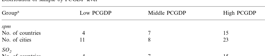
Table 1
Distribution of sample by PCGDP level
All
Groupa Low PCGDP Middle PCGDP High PCGDP
spm
No. of countries 4 7 15 26
No. of cities 11 8 23 42
SO2
No. of countries 4 7 15 26
No. of cities 10 8 21 39
aAs per World Bank guideline.
As regards the country-wise per capita income data, we have used the Summers and Heston country-wise real per capita GDP (measured at a common set of international prices) available from the Penn World Tables (Summers and Hes-ton, 1988, 1991). It should be mentioned that the Summers and Heston real GDP data are available up to 1988, whereas the country-wise data on air pollution are available up to 1990. For the years 1989 and 1990, we have used the World Bank’s country-wise data on nominal per capita GDP after dividing these by the ratio of the Summers and Heston GDP data and the corresponding World Bank (1988) data in order to index-link the World Bank data for 1989 and 19905 (World
Bank, 1989, 1990). Since the pollution data are available city-wise for individual countries, ideally we should have some measure of city-wise per capita income. However, such income data being unavailable, we have used the real per capita GDP of the country (to which a specific city belongs) as a proxy for the per capita income of a city. Thus, for all the cities belonging to a coun-try, the same country level per capita income has been used. As the city-wise pollution data are available separately for three time periods as al-ready mentioned, we have used the average of yearly per capita incomes for a specific time-pe-riod as the measure of per capita income of that time period. Thus, the data set we have used in the present study is essentially of the nature of a panel data consisting of 42 cities in 26 countries
and three time-periods.6Note that of the 26
coun-tries represented in our data set, 15 belong to the high-income group. Thus, the present data set has a somewhat biased representation of countries with high income. Table 1 presents a two-way summary of the distribution of the countries and the cities by per capita income level (PCGDP) and pollutant type.
In our empirical analysis reported in this paper we have tried to explain the level of pollution in terms of production technique (as reflected by the capital – labour ratio for the economy as a whole) and sectoral composition of GDP of individual countries, in addition to PCGDP. Country-wise capital – labour ratios have been calculated on the basis of country-wise data on gross capital and employed labour force available in the United Nations National Income Accounts Statistics (1990) and ILO’s Yearbook of Labour Statistics, respectively. Finally, country-wise data on sec-toral composition of GDP have been obtained from the World Bank reports.
3. The regression set up and the results
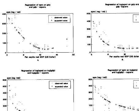
As already mentioned, the primary focus of the present study is on the relationship between ambi-ent air quality and real PCGDP. To examine the nature of this basic relationship, a number of alternative functional forms of the regression model have been tried, i.e.
Fig. 1. Relationship between PCGDP and spm.
yit=b0+b1xit+b2xit
2 (1)
yit=b0+b1lnxit+b2(lnxit)2 (2)
lnyit=b0+b1xit+b2xit2 (3)
lnyit=b0+b1lnxit+b2(lnxit) 2
(4) whereyitandxitdenote levels of air pollutant and real PCGDP for ith country at tth time period, respectively. These equations have been estimated for spm and SO2 separately for residential and
commercial locations at the three different time periods and also for the two types of locations combined and the three time periods combined.
The correlation coefficient between spm and real PCGDP was found to be negative and large
separately for each data set and also for the combined data sets. The smallest absolute value of this correlation is 0.79 (see Table 3). This finding contradicts the EKC hypothesis. However, such contradictory empirical results have been obtained earlier also. Grossman and Krueger (1993) and Torras and Boyce (1998) (and also Grossman and Krueger, 1995) reported results not supporting the EKC hypothesis for ambient spm and heavier particles, respectively.7 This is
confirmed if we look at the scatter diagrams, all of
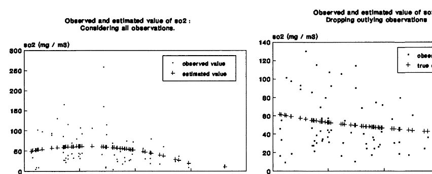
Fig. 2. Relationship between PCGDP and SO2.
Table 2
Distribution of countries by the level of PCGDP corresponding to turning point of EKC
Pollutants Group US$0–3000 US$3000–6000 US$6000–8000 US$8000 and more
spm c 6 7 1 20
r 8 2 0 4
All 14 9 1 24
SO2 c 8 14 7 20
3
r 5 10 2
All 13 24 9 23
which show the same decreasing pattern (see Fig. 1). A possible explanation of this may be the fact that the present data set contains observations relating to mostly developed countries (which may have crossed the so-called turning point of the EKC). Table 2, which gives the distribution of countries by selected level of PCGDP (assumed to correspond to the possible turning point of the EKC), may corroborate this. Thus, e.g. if the level of PCGDP corresponding to the turning point of the EKC for spm is taken to be US$8000, there 20 out of the 34 sample observations would belong to the declining portion of an inverted U-shaped EKC for spm.
As a part of the preliminary data analysis, we examined the summary statistics relating to the pollution data (i.e. mean and variance and corlation coefficient with PCGDP). These are re-ported in Table 3. It may be noted in this Table
that the average spm level for residential areas is higher than that for commercial areas, but the mean PCGDP level is higher for commercial areas than that for residential areas. This is possibly because of the fact that the residential areas in the present data set are mostly located in the less developed and developing countries.
Tables 4 – 6 present our regression results for spm. The scatter diagrams in Fig. 1A suggest that the shape of the underlying relationship between PCGDP and spm is U-shaped. The ordinary least squares (OLS) estimates of corresponding quadratic relationship between PCGDP and spm for different periods and areas are reported in Table 4. All these results show a negative value of
b1 and a positive value of b2, both of which are
statistically significant.8 Thus, for spm our results
8b
Table 3
Summary statistics of the suspended particulate matter for different groups and their combinationsa
Variance Correlation
Mean No. of countries
Group Variables
tis the group of countries with data from commercial areas of cities at timet, rr is the same from residential areas.
Table 4
Groupwise results of OLS regression for spm dataa
R2 (df) Estimated coefficients of explanatory variable
Group
'
Turning pointse2/n
e/n x2
Intercept x
0.36×10⁻⁵*** 0.93 (11) 32.30
419.43*** −0.073*** 25.37 10 033
c1
aNote: figures in parentheses are thet-ratios. Pollution is measured in mg/m3. Income is measured in terms of 1985 US dollars. * Coefficient estimate is significantly different from zero at 10%.
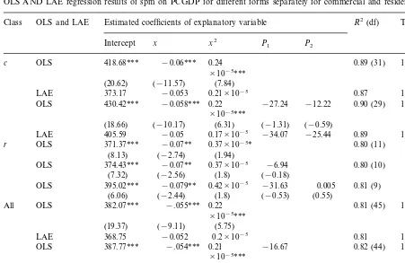
Table 5
OLS AND LAE regression results of spm on PCGDP for different forms separately for commercial and residential areasa
Estimated coefficients of explanatory variable R2(df)
Class OLS and LAE Turning points
P2
aNote: figures in parentheses are thet-ratios. Pollution is measured in mg/m3. Income is measured in terms of 1985 US dollars * Coefficient estimate is significantly different from zero at 10% level.
** Coefficient estimate is significantly different from zero at 5% and level. *** Coefficient estimate is significantly different from zero at and 1% level.
suggest a U-shaped relationship between spm and PCGDP, which implies that beyond a certain level of PCGDP (US$12 500), a further rise of PCGDP can be achieved at the cost of environ-mental degradation. 9
Clearly, this result
contra-dicts the usual EKC hypothesis, but supports some earlier findings. For example, Kaufmann et al. (1998)10 found U-shaped relationship between
income and atmospheric concentration of SO2
with a turning point around the PCGDP level of US$12 000; Sengupta (1997) noted that beyond the per capita income US$15 300, the environ-mental base (particularly carbon emissions) relinks with economic growth11
; and Shafik (1994), Grossman and Krueger (1995) obtained upward rising curves by fitting cubic relationships. It may be mentioned that our OLS diagnostics indicated presence of heteroscedasticity in the present data set. We therefore re-estimated all the
9An alternative measurement also reveals the same result. Instead of PCGDP, we took Gross City Product Per Capita (GCPPC) from World Resources 1998 – 99 (World Resources Institution et al., 1998). Using GCPPC and spm (mg/m3) for the year 1993, we found the same result, i.e. U-shaped relationship between spm and GCPPC. This later data set covered 22 cities across the world. The estimated relationship is: spm=215.4 (7.5)−0.01906(GCPPC) (-2.755)+0.416×10⁻⁶ (GCPCDP)2 (2.001). and the coefficients of GCPPC and square of GCPPC are significant at 5 and 10% level, respectively. In case of SO2, after removing an outlier, we obtained negatively sloped linear relationship. See Sukla and Parikh (1992).
S
.
Dinda
et
al
.
/
Ecological
Economics
34
(2000)
409
–
423
417
OLS regression results of spm on GDP and different dummy variables for different groups and their combination
R(2 R2(df) Group Estimated coefficient of explanatory variable
Z2 d1 d2 W1 W2 Z1
Intercept X P1 P2
−0.01* 0.81 (28)
c 318.4*** −0.018*** 23.65 23.64 −0.012** 0.78
(−1.77) (−2.24)
(o.43) (7.54) (−4.68) (0.45)
−32.36 0.73 (31) 0.71
311.5*** −0.02***
(−1.08) (−5.82)
(14.06)
356.2*** −0.03*** −209.4*** 0.02*** 0.82 (30) 0.80
(−4.07) (3.92)
(−7.87) (16.5)
−320*** 0.047**
418.7*** −0.051*** 0.91 (30) 0.90
* (−8.19) (6.29) (−7.38)
(18.35)
474.3** −0.07* −262.67 0.054 0.053 0.51 (8) 0.21
r −227.5
(1.39) (1.4)
(2.7) (−1.92) (−1.3) (−1.118)
340.2*** −0.0004 −282.7*** 0.93 (11) 0.92
(−9.37) (16.67) (−0.14)
−218.08*** −0.04* 0.95 (10) 0.93 281.5*** 0.037*
(−4.97) (1.88)
(7.77) (1.84)
−296** 0.05** 0.68 (10) 0.59
−0.057*** 377.9***
(6.4) (−3.437) (−2.96) (2.92)
−0.006 0.60 (42)
−0.008 0.56
288.1***
All −0.017*** 12.6 7.28
(−1.21)
(6.16) (−3.47) (0.21) (0.12) (−0.83)
−107.42***
297.2*** −0.014*** 0.69 (45) 0.67
(−4.12) (−4.57)
(15.3)
−273.26*** 0.03*** 0.83 (44) 0.82 363.8*** −0.031***
(−8.2) (6.13)
(−8.62) (20.15)
−317*** 0.05***
406.8*** −0.054*** 0.81 (44) 0.80
(−7.39) (6.28) (16.23) (−7.3)
aNote: pollution is measured in mg/m3. Income is measured in terms of 1985 US dollars. Figures in parentheses are thet-ratios. * Coefficient estimate is significantly different from zero at 10% level.
Table 7
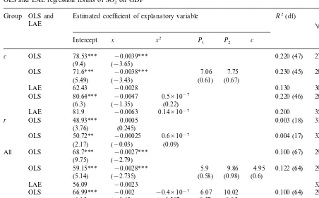
OLS and LAE regression results of SO2on GDPa
Group OLS and Estimated coefficient of explanatory variable R2(df)
'
e2/n e/n
c 0.220 (47) 27.96 22.86
(9.4) (−3.65)
71.6*** −0.0038*** 7.06 7.75
OLS 0.230 (45) 28.42 23.06
(5.49) (−3.43) (0.61) (0.67) 62.43 −0.0028
LAE 0.130 30.39 22.45
80.64*** −0.0047 0.5×10⁻⁷
OLS 0.220 (46) 28.25 22.72
(6.3) (−1.35) (0.22) 81.9 −0.0063 0.14×10⁻⁷
LAE 0.200 35.41 32.95
48.93*** 0.0005 OLS
r 0.003 (18) 31.98 24.8
(3.76) (0.245)
50.72** −0.00025 0.6×10⁻⁷
OLS 0.004 (17) 32.89 24.65
(2.17) (−0.03) (0.09) 68.7*** −0.0027***
OLS
All 0.100 (67) 29.63 24.65
(9.75) (−2.79)
59.15*** −0.0028*** 5.9 9.86
OLS 4.95 0.122 (64) 29.99 24.65
(5.14) (−2.735) (0.58) (0.98) (0.6) 56.09 −0.0023
LAE 32.88 23.25
66.99*** −0.002 −0.4×10⁻⁷ 6.07 10.02
OLS 0.100 (64) 29.84 24.65
(6.15) (−0.65) (−0.207) (0.57) (0.95)
OLS 59.5*** −0.003 0.13×10⁻⁷ 4.98 0.123 (65) 30.23 24.37
(4.54) (−0.88) (0.06) (0.6)
54.05 −0.002 −0.2×10⁻⁷
LAE 28.31 23.24
aNote: pollution (SO
2) is measured in mg/m3. Income is measured in terms of 1985 US dollars. Figures in parentheses are the t-ratios. Two and three asterisks indicate that estimated coefficient are statistically significant at 1 and 5% level, respectively.
regression specifications using the least absolute error (LAE) method.12 The estimated LAE and
OLS results are presented in Table 5. As is to be expected, the estimated LAE results are similar to the corresponding OLS results. Perhaps the most interesting findings for spm again are the U-shaped relationship with rather high PCGDP val-ues corresponding to the turning point (vide last columns of Tables 4 and 5). This is in contrast to the results of Selden and Song (1994), Grossman and Krueger (1995), who observed a turning point for spm around PCGDP levels of US$8000 and 5000, respectively. To be precise, our turning point estimates for spm vary between US$9500 and 14 000.
Table 5 presents the estimated OLS and LAE results for commercial, residential areas separately and also for the combined data for the two types of areas. So far as these estimates are concerned, it should be noted that the OLS and the corre-sponding LAE estimates are broadly similar, both in terms of goodness of fit and magnitude of the estimated parameters (however, unique LAE esti-mate could not be obtained in specific cases). A closer look at Table 5 may suggest the following results. First, the values of R2 and the PCGDP
corresponding to the turning point for residential areas are smaller than those estimated for com-mercial areas. Next, while the estimated coeffi-cients of PCGDP (i.e. b1) are negative and
those of square of PCGDP (i.e.b2) are positive in
all the cases, the estimated b2 coefficients for
residential areas are not highly significant. Thus, statistically speaking, the U-shape of the Pollu-tion – PCGDP relaPollu-tionship is weaker for the data
relating to the residential areas, but is rather strong for the data relating to the commercial areas. The estimated values of PCGDP corre-sponding to the turning point are estimated to be
US$9500 and 12 500 for residential and
com-mercial areas, respectively.13
Interestingly, the high-income countries observed to lie beyond the turning point in the present exercise included the USA, Canada, Japan, Finland and Germany. One might seek an explanation of difference in the results for the two types of areas in terms of how the relative density of population in these two types of areas changes with economic growth.
In the next part of the exercise an attempt was made to have a causal explanation of the ob-served U-shaped/inverse pollution – PCGDP rela-tionships. A priori, one should expect the pollution level in an economy to depend not only on the level of PCGDP, but also on the sectoral composition of GDP, how the PCGDP level is being achieved, and the time rate of growth of PC GDP. The sectoral composition is important, be-cause, ceteris paribus, an economy with a larger industrial production is likely to have more pollu-tion. The nature of the production technique used may be relevant, because often a more capital-in-tensive production technique is likely to be more non-human, energy-intensive and hence more pol-luting. Finally, the rate of growth of PCGDP may be a determining factor since, ceteris paribus, a faster growth may commonly be achieved by exer-cising the softer option of using more polluting production practices. In other words, a strong urge to grow faster, given the level of PCGDP, may induce a less developed economy to adopt a less clean production technique. Coming to the possible partial effect of production technique (as represented by the capital – labour ratio) of an
economy, say, it may be argued that between two countries with the same level of PCGDP, one having a greater concern for pollution would have a higher capital – labour ratio, if a cleaner technol-ogy is more capital intensive.14 Thus, we tried to
examine the validity of the following hypotheses (i) the marginal change in pollution level with respect to PCGDP is increasing in the rate of growth of PCGDP and decreasing in time; and (ii) the marginal change in pollution level with respect to PCGDP is decreasing in both the capital – labour ratio and the sectoral composition of GDP. To examine the possible partial effects of production technique and sectoral composition of GDP on pollution, the following regression set up was used:
yit=b0+b1xit+g1p1+g2p2+d1z1+d2z2+h1d1
+h2d2+u1w1+u2w2+eit (5)
where yit and xit are as already defined; pj is the dummy variable representing time period (i.e.
p1=l for the period 1979 – 1982 and zero
other-wise, p2=1 for period the 1983 – 1986 and zero
otherwise); d1 is the dummy variable for capital
intensity (i.e.d1=1 for a country having capital –
labour ratio greater than or equal to 1 and zero otherwise); d2 is the dummy variable for share of
non-agricultural sector in GDP (i.e. d2=1 for a
country for which the non-agricultural sector ac-counts for 90% or more of GDP and zero other-wise); zj=x*pj, j=1, 2 are the income – time period interaction terms; w1=x*d1 is the
in-come – capital intensity interaction term; w2= x*d2 is the income-share of non-agricultural
sector interaction term; and eit is the equation disturbance term.
Let us first discuss the results relating to the effects of capital intensity and sectoral composi-tion of GDP on the pollucomposi-tion level. Table 6 presents these results for spm. So far as the level of spm (i.e. the intercept term of the regression of
13These figures are higher than those found in the studies of Shafik and Banerjee (World Development Report 1992); Selden and Song (1994), Shafik (1994), Grossman and Krueger (1995). Kaufmann et al. (1998), on the other hand, found a U-turn for the atmospheric concentration of SO2at PCGDP level US$12 000. Grossman and Krueger (1995) also ob-served an upswing of the pollution level at about a PCGDP level of US$16 000. However, because there were only two observations beyond these levels, existence of such a reverse upswing at high level of PCGDP was not claimed.
Table 8
Estimated coefficients of Eq. (6)
R2(df)
Estimated coefficients of explanatory variable R(2
x x2 g g2
spm level on PCGDP) is concerned, in none of the equations the coefficients of the time dummy variables were statistically significant, implying thereby that the level of spm did not shift percep-tibly over time. As regards the effect of capital intensity on the spm level (i.e. the intercept dum-mies for this variable), this was observed to be negative and highly significant for the data relat-ing to the residential areas and the combined data, but non-significant for the data relating to the commercial areas. A similar significant nega-tive level effect of the sectoral composition vari-able was also observed for all the three data sets. Let us next describe the results showing how the marginal change in pollution in response to a change in the level of PCGDP (i.e. the slope term of the regression of spm level on PCGDP) are affected by the time dummy, capital intensity and the sectoral composition variables. These are given by the estimated values of the parameters associated with the interaction terms of PCGDP and these variables (i.e. the values of the parame-ters d1 and d2 measuring the effect of interaction
between time and PCGDP, u1 measuring the
ef-fect of interaction between capital intensity and PCGDP, and u2 measuring the effect of
interac-tion between sectoral composiinterac-tion of GDP and PCGDP, respectively, in Eq. (5)). The interaction effect between time and PCGDP is negative and significant only for the data relating to the com-mercial areas. This implies that compared to 1979 – 82 in latter periods the decrease in pollution in response to a marginal increase in PCGDP was greater. Next, the interaction effect between capi-tal intensity and PCGDP is positive and highly significant for the data relating to the commercial areas and also for the combined data. For the data relating to the residential areas this effect is,
however, negative and significant at 10% level. The positive interaction effect suggests that, ce
-teris paribus, a country with a higher capital
in-tensity would have a lower, but flatter, pollution – PCGDP curve compared to one with a lower capital intensity.
Finally, the interaction effect between sectoral composition of GDP and PCGDP was estimated to positive and significant for all the three data sets. This, together with the fact that the coeffi-cient of the corresponding intercept dummy is negative and significant, suggests that, ceteris
paribus, more industrialised countries have a
lower, but flatter, pollution – PCGDP curve. In this context it may be mentioned that for all the data sets the goodness of fit of the quadratic pollution – PCGDP equation is more or less simi-lar to those of the corresponding regression equa-tion in which PCGDP, capital intensity (sectoral composition of GDP) and interaction between PCGDP and capital intensity (sectoral composi-tion of GDP) are used as separate regressors. This possibly means that in association with PCGDP structural factors like production technique and sectoral composition may help explain observed changes in pollution level over time or across region. In other words, the quadratic term on the r.h.s. of Eq. (1) is in fact replaced by (g1p1+ g2p2+d1z1+d2z2+h1d1+h2d2+u1w1+u2w2) to
yield Eq. (5), because a priori rate of change of marginal pollution due to PCGDP level may be due to the total effects of technology, sectoral composition of GDP, time and their interaction with income level.
yit=b0+b1xit+b2xit 2
+a1git+a2git 2
+c(xitgit)
+eit (6)
whereyit,xit andeit are as already defined andgit
denotes the rate of growth of PCGDP for theith country at timet. It should be mentioned that for each individual country in the sample average growth rate of PCGDP for the three sub-periods, i.e. 1979 – 82, 1983 – 86 and 1987 – 90, were com-puted so that the value of gitwould be the average
growth rate for the period to which the year t
belonged.
The regression equation specified above was estimated for the combined data set alone. The estimated equation is presented in Table 8. As may be seen from the Table 8, the overall fit of the regression equation is fairly satisfactory. The estimated coefficients, except the one associated with the growth rate variable git, are all
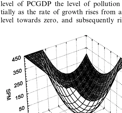
statisti-cally significant. The quadratic form of this rela-tionship suggests that, given a rate of growth, the pollution – PCGDP relationship is inverse or even U-shaped. On the other hand, given a PCGDP level, the quadratic pollution – growth relationship suggests a U-shaped relationship between the two variables. To be more specific, at a relatively high level of PCGDP the level of pollution falls ini-tially as the rate of growth rises from a negative level towards zero, and subsequently rises when
the rate of growth crosses a threshold level. At a relatively low level of PCGDP, however, pollution increases much faster with growth beyond a threshold level. A diagrammatic representation of the estimated pollution – PCGDP – growth equa-tion is presented in Fig. 3.
The results of the analysis of our SO2pollution
data are summarised in Table 7. Compared with the analysis of the spm data, fewer interesting findings are obtained in this case. To be precise, while the correlation coefficients between SO2and
PCGDP were observed to be negative for data sets relating to commercial areas, the correspond-ing correlation coefficients for residential areas were observed to be positive. This may be due to the fact that the data set for residential areas included data for only three developed countries, i.e. USA, Canada and the New Zealand, whereas the data set for commercial areas covered, in addition to these three countries, a number of other developed countries. Examination of the scatter diagrams suggested wide variation of the SO2level at low level of PCGDP which gradually
narrowed down as the PCGDP level increased. Further probe suggested presence of some outliers (i.e. data relating to Iran and Italy) in the data set, which were dropped in subsequent analyses.15
Removal of these outliers resulted in a linear relationship with a negative slope (not an inverted U-shaped relationship) between SO2 level and
PCGDP (see Fig. 2B). These results thus suggest absence of any clear relationship between the level of SO2 and PCGDP for data relating to the
residential areas. A possible explanation of the observed relationship for commercial areas could be that the extent and the quality of automobile emission improved considerably with rise in PCGDP.16
In addition, the type of fuel used for domestic and commercial purposes in low income developing countries might contribute to the rela-tively high level of atmospheric SO2in them. With
economic growth a transitional force strengthens the market mechanism and as a result the
econ-Fig. 3. Spm level vs. per capita GDP and economic growth.
15The data for Iran was unusual possibly because of the Iraq – Iran war during 1977 – 88, whereas Italy experienced a series of volcanic eruptions during the early 1980s.
omy gradually shifts from non-commercial to commercial energy resources. There may also be another reason, i.e. high income countries tend to spend more on defensive expenditure, enforce a stricter environmental regulation and use cleaner technology which others cannot afford.
4. Conclusion
The basic objective of the present study was to re-examine the hypothesis of EKC using cross-country time series data on two air pollutants, i.e. spm and SO2. Our results do not support the
EKC hypothesis. In contrast, for SO2we obtained
an inverse relationship with PCGDP, while for spm a shaped, rather than an inverted U-shaped, relationship with PCGDP is observed with an upward turn of the curve around a PCGDP level of US$12 500, which represents a rather high level of material consumption. To the extent the level of currently available technology is unable to ensure sustainability of such a high consumption level, a further rise of PCGDP be-yond the threshold level can support consumption only at the cost of a slow but steady deterioration of the environmental quality.
To explain the observed pollution – PCGDP re-lationship, three economic variables other than PCGDP were brought into the analysis i.e., the economy-level capital intensity, the sectoral com-position of GDP, and the rate of growth of GDP. It was thought that, given the PCGDP level of an economy, these three aspects would determine the exact nature of relationship that might exist be-tween pollution and income level. In other words, it is not only the level of income but also the characteristics of an economy which together de-termine the rate of environmental degradation that an economy will experience as it moves along the trajectory of development. Although the way these variables have been used in the present study leaves scope for improvement, their inclu-sion does give meaningful and statistically signifi-cant results so far as the explanation of the phenomenon of pollution is concerned. Briefly, our results suggest that the partial effect of capital intensity on pollution is generally negative (which
may not be unreasonable, if the trend of techno-logical progress is such that more capital-intensive techniques are more environment-friendly and vice versa). The observed negative partial effect of the sectoral composition variable on pollution perhaps suggests that, given the PCGDP level, the more industrialised an economy is, the lower and flatter would be its pollution – PCGDP curve. Fi-nally, PCGDP and the rate of growth variable seem to be jointly important in explaining ob-served pollution level of an economy.
Acknowledgements
We are grateful to two anonymous referees of this journal for helpful comments on earlier drafts of this paper.
References
Agras, J., Chapman, D., 1999. A dynamic approach to the environmental Kuznets curve hypothesis. Ecol. Econ. 28, 267 – 277.
de Bruyn, S.M., van den Bergh, J., Opschoor J., 1998, Eco-nomic growth and emissions: reconsidering the empirical basis of environmental Kuznets curves. Ecol. Econ. 25, 161 – 75.
Carson, R.T., Jeon, Y., McCubbin, D.R., 1997. The relation-ship between air pollution emissions and income: US data. Environ. Dev. Econ. 2, 433 – 450.
Cole, M.A., Rayner, A.J., Bates, J.M., 1997. The environmen-tal kuznets curve: an empirical analysis. Environ. Dev. Econ., 2, 401 – 416.
Grossman, G., Krueger, A., 1993. Environmental impacts of a North American free trade agreement. In: Garber, P. (Ed.), The Mexico – US Free Trade Agreement. Cambridge, MA: MIT Press.
Grossman, M.G., Krueger, A.B., 1995. Economic growth and the environment. Q. J. Econ. 5, 353 – 377.
Holtz-Eakin, D., Selden, T.M., 1995. Stocking the fires? CO2 emission and economic growth. J. Public Econ. 57, 85 – 101.
Judge, G., Griffiths, W.E., Hill, R.C., Lutkepohl, H., Lee, T.-C., 1985. The Theory and Practice of Econometrics, 2nd edn. Wiley, New York.
Kahn, M.E., 1998. A household level environmental Kuznets curve. Econ. Lett. 59, 269 – 273.
Komen, M.H.C., Gerking, S., Folmer, H., 1997. Income and environmental R&D: empirical evidence from OECD coun-tries. Environ. Dev. Econ. 2, 505 – 515.
McConnell, K.E., 1997. Income and the demand for environ-mental quality. Environ. Dev. Econ. 2, 383 – 399. Moomaw, W.R., Unruh, G.C., 1997. Are environmental kuznet
curves misleading us? The case of CO2emmissions. Environ. Dev. Econ., 2, 451 – 463.
Panayotou, T., 1997. Demystifying the environmental Kuznets curve: turning a black box into a policy tool. Environ. Dev. Econ. 2, 465 – 484.
Rothman, D.S., 1998. Environmental Kuznets curve — real progress or passing the buck?: A case for consumption-based approaches. Ecol. Econ. 25, 177 – 194.
Selden, T.M., Song, D., 1994. Environmental quality and development: is there a Kuznets curve for air pollution emissions? J. Environ. Econ. Manag. 27, 147 – 162. Sengupta, R.P., 1997. CO2emission – income relationship:
pol-icy approach for climate control. Pac. Asia J. Energy 7 (2), 207 – 229.
Shafik, N., 1994. Economic development and environmental quality: an econometric analysis. Oxf. Econ. Pap. 46, 757 – 773.
Sukla, V., Parikh, K., 1992. The environmental consequences of urban growth: cross-national perspectives on economic development, air pollution, and city size. Urban Geogr. 13 (5), 422 – 449.
Summers, R., Heston, A., 1988. A new set of international comparisons of real product and price levels: estimates for 130 countries, 1950 – 1985. Rev. Income Wealth 34 (1), 1 – 25. Summers, R., Heston, A., 1991. The Penn World Tables (mark V): an expanded set of international comparisons, 1950 – 1988. Q. J. Econ. 106 (2), 327 – 368.
Suri, V., Chapman, D., 1998. Economic growth, trade and energy implications for the environmental Kuznets curve. Ecol. Econ. 25, 195 – 208.
Torras, M., Boyce, J.K., 1998. Income, inequality, and pollu-tion: a reassessment of the environmental Kuznets curve. Ecol. Econ. 25, 147 – 160.
United Nations National Income Accounts Statistics, 1990. Parts I and II, United Nations Publication.
Vincent, J.R., 1997. Testing for environmental Kuznets curves within a developing country. Environ. Dev. Econ. 2, 417 – 431.
World Bank, 1988. World Development Reports. Oxford Uni-versity Press, Oxford (also other issues).
World Bank, 1989. World Development Reports. Oxford Uni-versity Press, Oxford (also other issues).
World Bank, 1990. World Development Reports. Oxford Uni-versity Press, Oxford (also other issues).
World Bank, 1992. World Development Report, Special issue on Development and the Environment. Oxford University Press, Oxford.
World Resources Institution, UNDP, UNEP, World Bank 1998, World Resources, 1998 – 99, Oxford University Press, Oxford.
Further Reading
Fields, G.S., Jakubson,G.H., 1994, New evidence on the Kuznets curve. Cornell University (mimeo).
Kuznets, S., 1955. Economic growth and income inequality. Am. Econ. Rev. XLV, 1 – 28.