Tabel Kontingensi 2x2 (4)
Uji Kebebasan untuk Data Ordinal
Uji Eksak untuk Ukuran Contoh Kecil
Uji Kebebasan
Chi-Squared χ
2dan G
2Data Nominal pada kolom dan
Squared χ dan G
barisData ordinal pada
Data ordinal pada
Uji Kecenderungan Linier
Peubah
ordinal
Asosiasi
tren
X ↑ÆY↑
X↑ÆY↓
Uji Kecenderungan Linier
• u1 ≤ u2 ≤ · · ·≤ ui
Æ
skor baris, dan
• v1 ≤ v2 ≤ · · · ≤ vj Æ skor kolom
• Urutan skor sama dengan level kategori
• Dengan dan
i i iu
=
∑
u p
+ j j jv
=
∑
v p
+• Korelasi
• Hipotesis
H0: Peubah baris dan kolom saling bebas vs
Ha: ρ ≠ 0,
k 2 ( ) 2
• Statistik Uji : M2= (n − 1)r2
• Untuk nilai n yang besar, M2mendekati sebaran
chi-squared dengan db= 1.
• M = √(n − 1)r, mengikuti sebaran normal baku. Pada hipotesis alternatif satu arah, seperti Ha :ρ > 0.
• Seperti pada χ2 dan G2, M2pun tidak memperhatikan
mana peubah respon/penjelas
Ilustrasi: Alcohol Use and Infant Malformation
• prospective study of maternal drinking and congenital malformations.
• After the first 3 months of pregnancy, the women in the sample completeda questionnaire about alcohol consumption.
• Following childbirth, observations were recorded on the presence or absence of congenital sex organ malformations.
• Alcoholconsumption, measured as average number of drinks per p , g p day, is an explanatory variable with ordered categories.
df 4 G
26 2
df = 4, G
2= 6.2
(P =
0.19
)
df = 4, X
2= 12.1
(P =
0.02
)
Dengan uji kecenderungan linier
• v1 = 0, v2 = 0.5, v3 = 1.5, v4 = 4.0,v5 = 7.0, skor
terakhir ditentukan secara sembarang
terakhir ditentukan secara sembarang.
• r = 0.0142.
• Statistik Uji M
2= (32,573)(0.0142)2 = 6.6
memiliki P-value = 0.01, berarti cukup bukti
mengatakan bahwa ada korelasi (nonzero
l ti
)
correlation).
• Statistik normal baku M = 2.56 memiliki P =
0.005 untuk Ha: ρ > 0.
Syntax SAS untuk menghitung M
2DATA alcohol;
INPUT item1 $ item2 $ row col count; DATALINES; DATALINES; strongagree strongagree 1 1 97 strongagree agree 1 2 96 ... ... strongdis strongdis 4 5 2 ;
/*For the TABLES command, use the numeric variables that contain the row and column scores.*/
PROC FREQ;;
TABLES row*col / chisq measures;
■ membaca output output:
◆ “Mantel-Haenszel Chi-Square” adalah M2(untuk skor dengan jarak yang sama).
◆ “Pearson correlation” adalah r.
Bagaimana menentukan skor yang
tepat?
Alkohol i
Skor SkorSkorSkor consumption 0 1 <1 2 1-2 3 3-5 4 6 5
M
2= 1.83,
(P = 0.18)
0 1 2 3 2 4 6 8 10 20 30 40 ≥6 105045Alternatif Æ Midrank sebagai skor
Alcohol consumpt
ion
Malformation Total kum Midrank
Absent PresenKonsekwensinya adalah t
0 17066 48 17114 17114 (1+17114)/2= 8557,5
<1 14464 38 14502 31616 (17,115 + 31,616)/2= 24,3655
1-2 788 5 793 32409 (31617+32409)/2= 32013 bahwa skema penilaian ini memperlakukan
tingkat konsumsi alkohol 1-2 (kategori 3) lebih dekat dengan tingkat konsumsi ≥6 (kategori 5) daripada tingkat konsumsi 0
(kategori 1).
3-5 126 1 127 32536 (32410+32536)/2= 32473
≥6 37 1 38
M
2 32574= 0,35,
(32537+32574)/2= 32555,5(P = 0.55)
Sytntax Sas untuk midranks
PROC FREQ;
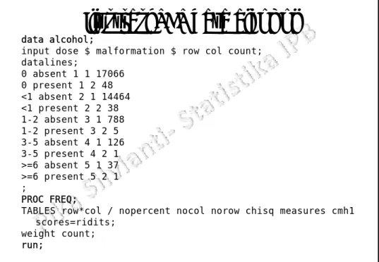
Ilustrasi SAS data alcohol
data alcohol;
input dose $ malformation $ row col count; datalines; 0 absent 1 1 17066 0 present 1 2 48 1 b 2 1 1 6 <1 absent 2 1 14464 <1 present 2 2 38 1-2 absent 3 1 788 1-2 present 3 2 5 3-5 absent 4 1 126 3-5 present 4 2 1 >=6 absent 5 1 37 >=6 present 5 2 1 ;; PROC FREQ;
TABLES row*col / nopercent nocol norow chisq measures cmh1 scores=ridits;
weight count; run;
• Statistik Uji M
2memperlakukan
kedua
klasifikasi sebagai ordinal
. Ketika satu variabel
(misalnya X) adalah nominal tetapi hanya
memiliki dua kategori, kita masih bisa
memiliki dua kategori, kita masih bisa
menggunakannya.
• Ketika X adalah nominal dengan lebih dari dua
kategori, uji ini tidak lagi sesuai untuk
digunakan.
Alternatif lain
gamma
Kendall’s tau-b
Cochran–Armitage
trend test
Dibahas pada• Uji Chi-square tidak valid jika ukuran contoh
l tif k il Æ l bih d i 25%
l
iliki il i
relatif kecil Æ lebih dari 25% sel memiliki nilai
harapan< 5 Æ
see WARNING under the result
of test.
• Saat n kecil, inferensia bisa dilakukan dengan
melihat exact distributions dibandingkan
g
large-sample approximations
Fisher’s Exact Test
(Uji Pasti Fisher)
Based on Hypergeometric distributionHipotesis nol pada uji pasti fisher adalah kedua
peubah (baris dan kolom) saling bebas
Uji Pasti Fisher (lanjutan)
• Uji pasti Fisher berlaku untuk semua ukuran contoh (tidak hanya untuk ukuran contoh kecil)
• Untuk ukuran contoh besar uji ini memerlukan waktu komputasi yang lama. Nilai-p yang dihasilkan akan mendekati nilai-p dari uji khi-kuadrat (chi-squared)
• Uji khi-kuadrat efisien jika ukuran contoh besar
Tabel 2x2
men women total Rasio odds
dieting a b a + b not dieting c d c + d totals a + c b + d n 11 22 12 21
ˆ
n n
n n
θ
=
Tahapan Uji Pasti Fisher
1. Susun Hipotesis H
0:p
1=p
22 B t t b l t b l
l bih “ k t i ” d
2. Buat tabel-tabel yang lebih “ekstrim” dengan
mengurangi pengamatan terkecilnya tetapi
jumlah baris dan kolomnya harus tetap
3. Hitung semua nilai p
iuntuk seluruh tabel
tersebut
4. Tentukan p
hit=p
1+p
2+p
3+p
4, dan tolak H
0jika
p
hit<α(uji 1 arah) atau p
hit<α/2(uji 2 arah)
Contoh Kasus
Seseorang ingin melihat hubungan antara pola diet seseorang dengan jenis kelamin. Uji pada taraf 5% seseorang dengan jenis kelamin. Uji pada taraf 5% apakah proporsi jenis kelamin pada yang melakukan diet dan yang tidak diet sama atau tidak
men women total
dieting 9 6 15
1
not dieting 3 4 7
Buat tabel lebih ekstrim…
men women total
dieting 10 5 15
men women total
dieting 11 4 15 dieting 10 5 15 not dieting 2 5 7 totals 12 10 22 dieting 11 4 15 not dieting 1 6 7 totals 12 10 22
men women total
3
2
dieting 12 3 15 not dieting 0 7 7 totals 12 10 224
Hitung semua p
i..
1 12!10!15! 7! 0.270897 22!9!3! 6! 4! p = = !9!3! 6! ! 3 12!10!15! 7! 0.014776 22!11!1! 4! 6! p = = 2 12!10!15! 7! 0.09752 22!10! 2!5!5! p = = 3 22!11!1! 4! 6! pP
hitdan keputusan…
Phit=0.270897+0.09752+0.014776+0.0007036307 =0 3839
=0.3839
Karena P
hit>0.025, maka terima H
0Æ Belum cukup bukti mengatakan
bahwa proporsi jenis kelamin pada bahwa proporsi jenis kelamin pada yang melakukan diet dan yang tidak diet berbeda
Ilustrasi
• To illustrate this test in his 1935 book, The Design of
Experiments, Fisher described the following
experiment: When drinking tea a colleague of Fisher’s experiment: When drinking tea, a colleague of Fisher s at Rothamsted Experiment Station near London
claimed she could distinguish whether milk or tea was added to the cup first.
• To test her claim, Fisher designed an experiment in which she tasted eight cups of tea. Four cups had milk added first and the other four had tea added first added first, and the other four had tea added first. • She was told there were four cups of each type and she
should try to select the four that had milk added first. • The cups were presented to her in random order.
• The null hypothesis H0: θ = 1 for Fisher’s exact test states that her guess was independent of the actual order of pouring.
• The alternative hypothesis that reflects her claim,
di i i i i i b d
predicting a positive association between true order of pouring and her guess, is Ha: θ > 1
Hipotesis
H0: θ = 1 vs Ha: θ > 1
Poured Guess Total
milk tea
Poured Guess Total
ilk t P = P(3) + P(4) = 0.243 Kesimpulan: Milk 3 1 4 tea 1 3 4 Total 4 4 8 milk tea Milk 0 1 4 tea 0 3 4 Total 4 4 8 Kesimpulan:
Kapena p> 0,05 berarti belum cukup bukti untuk menolak H0. Tidak ada asosiasi antara urutan menuang dengan tebakan
Syntax SAS
data tea;
input poured $ guess $ count; datalines; milk milk 3 milk tea 1 tea milk 1 tea tea 3 ;
proc freq data=tea;
p q
tables poured*guess/ nopercent nocol norow chisq; weight count;
exact pchi chisq or;
run;