Volume 25, Number 2, 2010, 129 – 142
TRADE SPECIALIZATION INDICES:
TWO COMPETING MODELS
Samsubar Saleh
Universitas Gadjah Mada ([email protected])
Tri Widodo
Universitas Gadjah Mada ([email protected])
ABSTRACT
Revealed Comparative Advantage (RCA) index by Balassa (1965) is intensively applied in empirical studies on countries’ comparative advantage or trade specialization. Asymmetric problem in the criteria of RCA index encourages Dalum et al. (1998) and Laursen (1998) to make Revealed Symmetric Comparative Advantage (RSCA) index. These two indexes are commonly employed in econometric models for analyzing countries’ trade specialization. This paper aims to compare theoretically and empirically the two competing econometric models, one using RCA and the other using RSCA. The ASEAN countries’ comparative advantages are presented for the empirical case studies. This paper concludes that RSCA can, to some extent, reduce the “outlier problem” of RCA in the econometric model; therefore, the model using RSCA can be more statistically reliable than the model using RCA. The two econometric models might not be suitable for forecasting purposes since the estimated values could theoretically violate their criteria of comparative advantage and disadvantage. In the cases of ASEAN countries, we find empirically that the model using RSCA is statistically more reliable than the one using RCA. The ASEAN countries have exhibited de-specialization.
JEL classification: F10, F14, F17
Keywords: Revealed Comparative Advantage (RCA), Revealed Symmetric Comparative Advantage (RSCA).
INTRODUCTION
Comparative advantages determine coun-tries’ trade specialization. In international trade theories, the concept of difference in comparative advantage is defined in term of autarkic (pre-trade) relative prices. Any difference in the autarkic relative prices be-tween two countries indicates the possibilities for them to gain from trade. Since the autarkic
relative prices are not observable in post-trade equilibriums, in empirical works the concept must be measured indirectly using post-trade data.
comparative advantage, i.e. the ratio of exports to production, the ratio of imports to consump-tion, the ratio of net trade to producconsump-tion, the ratio of production to consumption, the ratio of actual net trade to “expected” production, the ratio of the deviation of actual from expected production to expected production, the ratio of the deviation of actual from expected con-sumption to expected production, the ratio of the net trade from the total trade, the ratio of actual exports to expected exports(1), and the Donges and Riedel index(2). Several other empirical measures are the Michaely index (Michaely, 1962), net trade index (Bowen, 1983), the contribution to the trade balance (CEPII, 1983), and the χ2
measure (Archibugi and Pianta, 1992) (3). However, Revealed Comparative Advantage (RCA) index by Balassa (1965) is the most intensively applied one (e.g. Aquino, 1981; Crafts and Thomas, 1986; Peterson, 1988; Crafts, 1989; Porter, 1990; van Hulst et al., 1991; Amiti, 1999; Dowling and Cheang, 2000; Isogai et al., 2002; Ng and Yeats, 2003).
Several researchers, such as Volrath (1991), Dalum et al. (1998), Laursen (1998) and Wörz (2005), among others, have noted several shortcomings of the RCA index, especially when it is applied in an econometric model for analyzing countries’ dynamic com -parative advantage. Dalum et al. (1998) and Laursen (1998), therefore, recommend an index namely Revealed Symmetric Compara-tive Advantage (RSCA), which is, in fact, a simple transformation of RCA index. This paper aims to compare both theoretically and empirically the two competing econometric models commonly used in the empirical studies for analyzing countries’ dynamic comparative advantage: one using RCA and the other using RSCA. The rest of this paper is organized as follows. Part 2 exhibits the two
(1) Revealed Comparative Advantage (RCA) or Balassa index by Balassa (1965) is included in this category. (2) For this index, please see Donges and Riedel (1977). (3) For the good discussion on these indexes, please see
Laursen (1998).
empirical econometric models for analyzing countries’ dynamic comparative advantage. Part 3 describes the empirical results in the cases of the ASEAN (Association of South East Asian Nations) countries’ dynamic trade specialization. Finally, several conclusions are presented in Part 4.
THE ECONOMETRIC MODELS
1. The Generic model
A simple econometric model (1) is
com-comparative advantage of country i in product j for years T and 0, respectively, and εij
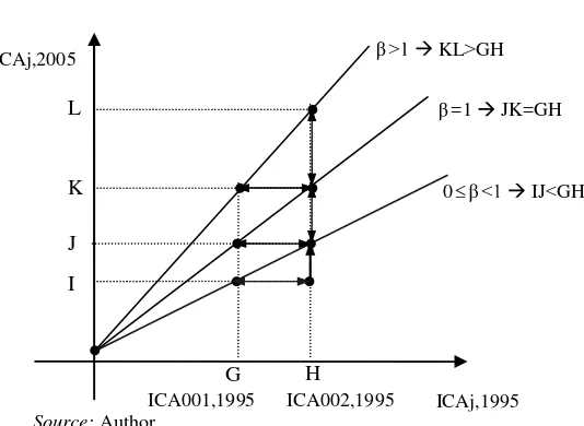
denotes white noise error term(4). The coefficient β specifies whether the existing trade specialization has been reinforced or not during the observation (Dalum et al., 1998; Laursen, 1998; and Wörz, 2005). To explain the specification, let us consider Figure 1, which describes the ICA for groups of products SITC (Standard International Trade Classification) 001 and SITC 002 in 1995 (horizontal axis) and 2005 (vertical axis), respectively. In the case of β is not signifi -cantly different from one (β=1), there is no change in the overall trade specialization. The difference between ICA001,1995 and ICA002,1995
(GH) equals the difference between ICA001,2005
and ICA002,2005 (JK). In the case of β>1, it
indicates the increase in specialization. The difference between ICA001,1995 and ICA002,1995
(GH) is smaller than the difference between ICA001,2005 and ICA002,2005 (KL). Finally,
0<β<1 indicates the de-specialization (IJ<GH) – that is, a country has gained comparative
advantage in industries where it did not specialize and has lost competitiveness in those industries where it was initially heavily specialized. In the event of β≤0, no reliable conclusion can be drawn on purely statistical grounds; the specialization pattern is either random, or it has been reversed.
To test statistically whether β equals one or not, we apply the Wald test. The statistic of the test is formulated as follows(5):
mk n R 1
R R F
2 UR
2 R 2 UR W
(2)
Where R2UR and R2R are the coefficients of determination of the unrestricted regression and the restricted regression, respectively(6); n is the number of observations (data); k is the
(5) See Intriligator et al. (1996) for the detailed explanation about the Wald coefficient restrictions test.
(6) The Wald test calculates the test statistic by estimating the unrestricted regression (subscript UR) and the restricted regression (subscript R)- without and with imposing the coefficient restrictions specified by the null hypothesis, Ho. The hypothesis are Ho:=1 and
Ho:≠1. The Wald statistic measures how close the
unrestricted estimates come to satisfying the restriction under the null hypothesis. If the restrictions are in fact true, then the unrestricted estimates should come close to satisfying the restrictions.
number of coefficients (including constant), and m is the number of restrictions. The statistic (ratio) FW is distributed following the
F distribution with m and n-k degree of freedom.
2. Two empirical measures of comparative advantage
There are many empirical measures of comparative advantage(7). Revealed Compara-tive Advantage (RCA) index by Balassa (1965) is the most intensively applied measure in many empirical works. The RCA index, which is also known as the Balassa index, is formulated as follows:
) x / x /( ) x / x (
RCAij ij in rj rn (3)
where RCAij stands for revealed comparative
of country i for group of products (SITC) j and xij denotes total exports of country i in group
of products (SITC) j. Subscript r represents all countries without country i, and subscript n refers all groups of products (SITC) except group of product j. The index represents a comparison of national export structure (the
(7) See, for example, Balance et al. (1987), Vollrath (1991) and Laursen (1998) for good discussions on several empirical measures of comparative advantage. ICAj,2005
ICA001,1995
G H
ICA002,1995 I
J K L
0 IJ GH
=1 JK=GH KL GH
ICAj,1995 Source: Author
numerator) with the world export structure (the denominator). The values of the index vary from 0 to infinity (0≤RCAij≤). RCAij
greater than 1 implies that country i has com-parative advantage in group of products j. In contrast, RCAij less than 1 means that country
i has comparative disadvantage in product j.
Since RCAij turns out to produce values
that cannot be compared on both sides of 1, the index is made to be a symmetric one. The new index is called Revealed Symmetric Comparative Advantaged (RSCA), which is formulated as (Dalum et al., 1998; Laursen, 1998):
) 1 RCA /( ) 1 RCA (
RSCAij ij ij (4)
RSCAij index varies from 1 to +1 (or
-1≤RSCAij≤1). The interpretation of RSCA is
similar with that of RCA. RSCAij greater than
0 implies that country i has comparative advantage in good j. In contrast, RSCAij less
than 0 implies that country i has comparative disadvantage in product j.
3. The two competing econometric models
In this paper, we examine two competing econometric models. The first model applies RCA in the above econometric model (1). The
model becomes:
ij 0 , ij T
,
ij RCA
RCA (5)
Where RCAij,Tand RCAij,0are the values of
RCA index country i in product j for years T and 0, respectively. εij denotes white noise
error term.
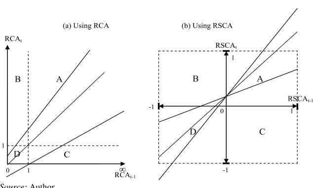
For the econometric model (5), several researchers, such as Dalum et al. (1998), Laursen (1998) and Wörz (2005), among others, have noted some shortcomings of RCA index, especially when it is applied in an econometric model for analyzing countries’ dynamic comparative advantages. First, RCA is basically not comparable on both side of unity since the index ranges from zero to infinity. A country is said not to be specialized in a given product if the index varies from zero to one. In contrast, a country is said to be specialized in a given product if the index ranges from one to infinity. Second, if RCA is used in estimating the econometric model, one might obtain biased estimates. RCA has disadvantage of an inherent risk of lack of normality. A skewed distribution violates the assumption of normality of the error term in regression analysis, thus not providing reliable inferential statistic. Third, the use of RCA in Source: Author
regression analysis gives much more weight to values above one, when compared to observa-tion below unity. In Figure 2 Panel (a), this is clearly shown by the much smaller quadrants Symmetric Comparative Advantage (RSCA) is more suitable for the econometric model:
ij
of RSCA index country i in product j for years T and 0, respectively. εij denotes white noise
error term.
4. Theoretical analysis
The use of either RCA or RSCA in the econometric model needs some considerations in the estimation. First, if RCA has disadvan-tage of an inherent risk of lack of normality, we would argue that the transformation from RCA to RSCA cannot guarantee automatically the normality distribution of RSCA; since the transformation is only a decreasing monotonic one(8). It is right that RSCA has symmetric criteria of comparative advantage with the central value 0, i.e. -1≤RSCAij≤1. However,
the symmetric in the criteria does not auto-matically guarantee the normality distribution of RSCA. Theoretically, a (continuous) ran-dom variable x, with the mean and the standard deviation has a normal distribution if its probability density function (pdf) has the following form:
See Hoy et al. (1995) for the detailed explanation on the monotonic transformation.
Although the ordinary least squares (OLS) does not require the normality distribution of the error terms, the assumption of normality is for the purpose of statistical inference. If RCA has disadvantage of an inherent risk of lack of normality, RSCA will also have the disadvan-tage since RSCA is only a decreasing mono-tonic transformation of RCA. Therefore, either non-normally distributed RCA or RSCA used in estimating the econometric model, one might obtain biased estimates.
Second, even if the mean of error terms is zero (E[ij]0) and there is no serial
correla-that the econometric equations (5) and (6) are ones of comparing two cross-sections at two points of time; i.e. there is no element of time in the observation. As the nature of cross-sections, we might face heteroscedastic. Therefore, the Ordinary Least Squares (OLS) might be not suitable for the estimation.
Third, since the linear econometric model is applied, the use of RSCA, as well as RCA, faces a problem of prediction or forecasting. There is no guarantee thatRSCA , the estimator
E(RSCAij,T|RSCAij,0), will necessarily fulfil
the restriction, -1≤RSCAij≤1. This problem where denotes rational number) while RCA is only bounded-below index (1≤RCAij≤, or
1,
RCA:1RCA
)(9). Figure 2 de-scribes this problem for the use of RCA (Panel a) and for the use of RSCA (Panel b) in the econometric model. When the RCA is used,(9)
See Hoy et al. (1995) for the detailed explanation
we might have such problem if only if the estimate constant (α) is negative, for any esti -mate coefficient in Equation 5. Meanwhile, we might have the problem for any estimate constant estimate constant (α) is negative, for any estimate coefficient in Equation 6. Therefore, we would suggest that analyzing the estimated values of RCA and RSCA (RCA
and RSCA
) is necessary before using the regres-sion for forecasting purposes.
THE EMPIRICAL ANALYSIS
1. Data
We use data on exports published by the United Nations (UN), namely the United
Nations Commodity Trade Statistics
Database (UN-COMTRADE). We choose the
3-digit SITC Revision 2 and focuses on 237 groups of products. The 3-digit SITC Revision 2 is chosen because it provides appropriately the detailed groups of commodities as well as the range of available data.
2. Are RCA and RSCA indexes normally theoretically transform from the non-normal distributed index to the normal distributed one. To examine this, we apply a formal test of the normality distribution, namely the Jarque-Bera (1987) (JB) test of normality on both RCA and RSCA. The JB statistic is formulated as distribution, the value of skewness is zero and the value of kurtosis is 3. Under the null hypothesis that the residuals are normally
distributed, Jarque and Bera (1987) show that asymptotically (i.e. in large sample) the statis-tic JB follows the chi-square distribution with degree of freedom 2 (
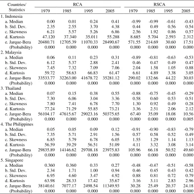
df22), which are equal to 7.779, 9.488 and 13.277 for the levels of significance 10%, 5% and 1%, respectively.Table 1 summarizes some statistics, in-cluding JB statistic, of both RCA and RSCA for the ASEAN countries for the periods 1987, 1985, 1995 and 2005. Since the transformation from RCA to RSCA is only a decreasing monotonic one, it is clearly shown in Table 1 that the median, standard deviation (Std.Dev.), skewness and kurtosis statistics of RSCA are always less than those of RCA. From the JB statistics, we can conclude that both RCA and RSCA are not normally distributed for all the ASEAN countries and for all the periods. However, in a specific case, the transformation could possibly change from the non-normally distributed RCA to the normally distributed RSCA, i.e. when the skewness and kurtosis are statistically equal to zero and 3, respectively.
3. Estimation methods
Heteroscedasticity might be in our estimation since the data applied in this paper is cross sectional one. However, the existence of autocorrelation also might be possible. The Ordinary Least Squares (OLS) might not suitable for the estimation. Hence, we employ Heteroscedasticity and Autocorrelation Con-sistent Covariance (HAC) when the usual OLS have violated the homoscedasticity or no-autocorrelation assumptions(10). There are two possible alternative approaches i.e. Heterosce-dasticity Consistent Covariance (HAC) White and HAC Newey-West. White (1980) formu-lated a heteroscedasticity consistent covari-ance matrix estimator which provides correct estimates of the coefficient covariances in the presence of heteroscedasticity of unknown
form. The White covariance matrix assumes that the residuals of the estimated equation are serially uncorrelated. Newey and West (1987) derived a more general estimator that is con-sistent in the presence of both heteroscedastic-ity and autocorrelation of unknown form.
4. Estimation results
Table 2 shows the estimation results of the econometric models (5) and (6), which are
given the headings M1 and M2, respectively, for the periods 1979-1985, 1985-1995, 1995-2005 and 1979-1995-2005 in the cases of five ASEAN countries i.e. Indonesia, Malaysia, the Philippines, Thailand and Singapore. Those periods are chosen to consider a short-period (6 years: 1979-2005), medium-periods (10 years: 1985-1995 and 1995-2005) and a long-period (26 years: 1979-2005). In general, we can say that almost all the estimation results Table 1. Some Statistics of RCA and RSCA of the ASEAN Countries:
1979, 1985, 1995, 2005 Countries/
Statistics
RCA RSCA
1979 1985 1995 2005 1979 1985 1995 2005
1. Indonesia
a. Median 0.00 0.01 0.24 0.41 -0.99 -0.99 -0.61 -0.43
b. Std. Dev. 2.35 2.55 3.70 4.38 0.44 0.49 0.56 0.54
c. Skewness 6.21 5.57 5.26 6.86 2.56 1.92 0.86 0.57
d. Kurtosis 47.120 37.340 35.011 55.288 8.685 5.704 2.593 2.312
e. Jarque-Bera 20480.71 12705.39 11070.33 28490.67 571.55 214.69 30.60 17.51
(Probability) 0.000 0.000 0.000 0.000 0.000 0.000 0.000 0.000
2. Malaysia
a. Median 0.06 0.11 0.23 0.31 -0.89 -0.81 -0.63 -0.53
b. Std. Dev. 6.12 5.37 2.88 2.41 0.46 0.47 0.49 0.47
c. Skewness 7.45 7.32 7.09 7.06 2.04 1.58 1.05 0.88
d. Kurtosis 59.72 58.63 66.83 61.47 6.61 4.89 3.38 3.05
e. Jarque-Bera 33533.77 32263.00 41678.72 35281.12 290.02 132.66 44.22 30.03
(Probability) 0.000 0.000 0.000 0.000 0.000 0.000 0.000 0.000
3. Thailand
a. Median 0.07 0.15 0.38 0.55 -0.88 -0.75 -0.45 -0.29
b. Std. Dev. 7.30 6.06 3.04 3.36 0.58 0.60 0.53 0.51
c. Skewness 7.80 7.41 6.78 7.70 1.30 0.92 0.49 0.28
d. Kurtosis 77.24 71.29 55.85 73.21 3.36 2.51 2.06 2.12
e. Jarque-Bera 56104.17 47615.67 29023.16 50375.65 67.40 35.09 18.08 10.56
(Probability) 0.000 0.000 0.000 0.000 0.000 0.000 0.000 0.005
4. The Philippines
a. Median 0.05 0.05 0.09 0.12 -0.91 -0.90 -0.83 -0.79
b. Std. Dev. 7.35 5.71 2.91 1.56 0.57 0.58 0.52 0.49
c. Skewness 6.85 5.79 6.78 6.05 1.55 1.29 1.14 1.13
d. Kurtosis 56.59 39.29 56.51 51.09 4.11 3.32 3.08 3.14
e. Jarque-Bera 29835.89 14146.62 29708.18 23975.83 105.96 66.18 50.52 49.60
(Probability) 0.000 0.000 0.000 0.000 0.000 0.000 0.000 0.000
5. Singapore
a. Median 0.360 0.360 0.33 0.27 -0.48 -0.47 -0.51 -0.58
b. Std. Dev. 2.34 1.71 1.00 0.94 0.46 0.45 0.43 0.42
c. Skewness 6.95 4.60 3.47 4.92 0.88 0.81 0.72 0.79
d. Kurtosis 63.98 28.33 17.42 35.67 3.16 3.11 2.83 2.96
e. Jarque-Bera 38140.61 7077.17 2498.54 11349.93 30.28 25.49 20.37 24.18
(Probability) 0.000 0.000 0.000 0.000 0.000 0.000 0.000 0.000
using both RCA (model M1) and RSCA (model M2) indicate de-specializations of the ASEAN countries’ comparative advantage. In the cases of Malaysia, the Philippines, Thailand and Singapore, all the coefficients in the both models M1 and M2 are statistically significant different from zero and different from one at the levels of significance 1%, 5% or 10%, excepting in the model M1 of Thailand for the period 1995-2005, which is equal to 1.01 (statistically not different from 1).
It is interesting to discuss further the estimation results of the models M1 and M2 in the case of Indonesia, since some of them give different or even opposite conclusions. For the period 1979-1985, the coefficients are 0.67 and 0.97 for the models M1 and M2, respec-tively. They are statistically significant differ-ent from zero, but statistically not differdiffer-ent from one. Although the coefficient of the model M1 is 0.67, it is statistically not different from one, because its standard deviation is relatively high. These coefficients indicate that Indonesia had lingered its specialization during that period. For the medium-term 1995-2005 and the long-term 1979-2005, the coefficients of the model M1 are 0.91 and 0.97, respectively, which are statistically significant different from zero but not different from one. Therefore, if we use the Model M1 for our analysis, we will conclude that during those periods Indonesian specialization had remained constant. Let us turn to the model M2 for the same periods. The model M2 gives the coefficients 0.83 and 0.57, respectively, which are both statistically significant different from zero and from one. Those figures imply that Indonesia had exhib-ited de-specializations during those periods. Here, we have two different conclusions from the Model M1 and M2. More surprisingly, the models M1 and M2 give opposite results for the period 1985-1995. The coefficient of the model M1 is 1.3, which is both statistically significant different from zero and from one; it
implies that Indonesia has increasingly specialized in its exports. On the contrary, that of the model M2 is 0.75, which is also both statistically significant different from zero and different from one; it implies that Indonesia had exhibited de-specialization.
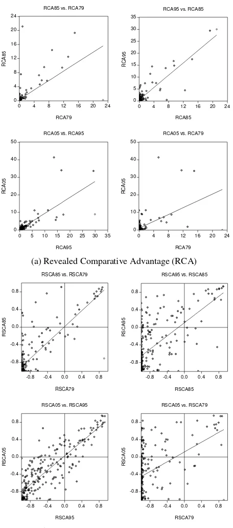
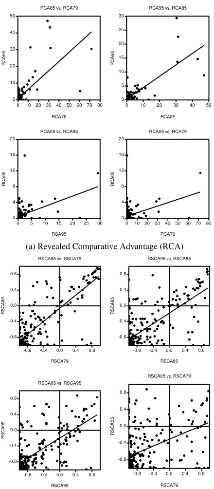
Hence, Indonesia is a good case study for comparing the two competing econometric model, one using RCA (model M1) and the other using RSCA (model M2). We would argue that such opposite conclusions happen due to the existence of “outlier problem” (11)
in RCA. Panel (a) in Figure 3 shows clearly this problem. So many groups of products (SITC) have RCA lower than 1; in contrast, only few groups of products have RCA greater than 1. Out of 234 groups of products (SITC), we find that there are only 20, 26, 55 and 62 groups of products (SITC) with RCA greater than 1 or even with very high values of RCA in 1979, 1985, 1995 and 2005, respectively(12). There is a sharp jump in the number of groups of products (SITC) with RCA greater than 1 in 1985-1995. Since the use of RCA in regres-sion analysis gives much more weight to values above one, when compared to observa-tion below one (Dalum et al., 1989; Laursen, 1989), such a sharp jump in the number of groups of products, here as the “outliers”, has affected the estimate.
(11) In the Boxplot analysis, for example, the outliers are defined as the values between 1.5 and 3 box lengths from the upper or lower edge of the box. The box length is the inter-quartile range. The values more than 3 box lengths from the upper or lower edge of the box
are referred to as “extreme” values.
Sa
leh &
Wid
o
d
o
137
Countries
Indonesia Malaysia the Philippines Thailand Singapore
Period/Estimates
M1 M2 M1 M2 M1 M2 M1 M2 M1 M2
1. Period 1979-1985
Constant (α) 0.33** 0.01 0.15* 0.02 0.60* -0.06 0.36* 0.03 0.24* -0.08**
(0.13) (0.06) (0.05) (0.03) (0.17) (0.05) (0.10) (0.04) (0.05) (0.03) Coefficient ( ) 0.67** 0.91* 0.85*,### 0.9*,# 0.56*,## 0.83*,# 0.76*,# 0.87*,# 0.65*,# 0.81*,#
(0.29) (0.06) (0.08) (0.03) (0.18) (0.05) (0.07) (0.04) (0.06) (0.05)
R-squared 0.39 0.68 0.94 0.78 0.52 0.65 0.84 0.73 0.8 0.67
Jarque-Bera Statistic of residual 37185.1 1030.1 22261.6 909.3 14651.1 409.0 14709.6 151.5 2829.6 253.7 (Prob. of Jarque-Bera) 0.000 0.000 0.000 0.000 0.000 0.000 0.000 0.000 0.000 0.000 2. Period 1985-1995
0.43* 0.1*** 0.46* -0.003 0.25* -0.19* 0.42* -0.08** 0.33* -0.15* (0.08) (0.05) (0.12) (0.03) (0.09) (0.05) (0.09) (0.03) (0.06) (0.03) Coefficient ( ) 1.3*,## 0.75*,# 0.44*,# 0.79*,# 0.41*,,# 0.66*,# 0.43*,# 0.60*,# 0.38*,# 0.7*,#
(0.13) (0.05) (0.09) (0.04) (0.10) (0.06) (0.07) (0.04) (0.08) (0.04)
R-squared 0.79 0.43 0.69 0.58 0.64 0.55 0.72 0.45 0.41 0.54
Jarque-Bera Statistic of residual 3742.8 13.8 6204.3 96.0 21094.7 129.3 9319.1 17.0 4872.4 46.3 (Prob. of Jarque-Bera) 0.000 0.001 0.000 0.000 0.000 0.000 0.000 0.000 0.000 0.000 3. Period 1995-2005
0.26 0.02 0.12* -0.05** 0.40* -0.20* 0.12 -0.01 0.12 -0.14*
(0.17) (0.02) (0.04) (0.02) (0.10) (0.05) (0.11) (0.03) (0.07) (0.22) Coefficient ( ) 0.91* 0.83*,# 0.79*,# 0.83*,# 0.26*,,# 0.64*,# 1.01* 0.73*,# 0.67*,## 0.80*,#
(0.24) (0.03) (0.07) (0.03) (0.09) (0.06) (0.11) (0.04) (0.16) (0.04)
R-squared 0.59 0.74 0.88 0.74 0.23 0.46 0.84 0.60 0.51 0.68
Jarque-Bera Statistic of residual 36121.0 13.5 30740.9 231.8 38570.8 116.9 5682.5 47.9 5003.7 9.5 (Prob. of Jarque-Bera) 0.000 0.001 0.000 0.000 0.000 0.000 0.000 0.000 0.000 0.009 4. Period 1979-2005
0.93* 0.11*** 0.57* -0.04 0.48* -0.31* 0.76* -0.08*** 0.42* -0.35* (0.18) (0.06) (0.10) (0.05) (0.10) (0.06) (0.10) (0.04) (0.07) (0.03) Coefficient ( ) 0.97*** 0.57*,,# 0.27*,# 0.59*,,# 0.09*,# 0.41*,# 0.30*,,# 0.34*,# 0.14***,# 0.34*,#
(0.51) (0.07) (0.08) (0.06) (0.01) (0.07) (0.07) (0.05) (0.08) 0.05
R-squared 0.27 0.22 0.48 0.33 0.16 0.22 0.43 0.15 0.12 0.13
Jarque-Bera Statistic of residual 20649.2 4.4 41533.5 25.6 35456.2 55.3 40584.8 6.0 6651.1 25.2
(Prob. of Jarque-Bera) 0.000 0.112 0.000 0.000 0.000 0.000 0.000 0.05 0.000 0.0000
Notes: M1 and M2 refer to the model with RCA (Equation 5) and the model with RSCA (Equation 6), respectively. Figures in parenthesis are standard errors. *,**,and *** mean statistically significant (different from zero) at the level of significances 1%, 5% and 10%, respectively. , and mean that the coefficient ( ) is statistically different from one (the Wald coefficient test) at the level of significances 1%, 5% and 10%, respectively.
# ## ###
0
(a) Revealed Comparative Advantage (RCA)
-0.8
(b) Revealed Symmetric Comparative Advantage (RSCA) Source: Author
Applying RSCA (in model M2), therefore, can at least reduce the outlier problem, as shown in Table 1 as well as in Panel (b) of Figure 3 in the case of Indonesia. From Table 1, we can firmly say that the distribution of RSCA always has a lower standard deviation (Std.Dev) than that of RCA; since the transformation from RCA to RSCA is, in fact, a decreasing monotonic one. Since RCA can vary from zero to infinity (0≤RCA≤), the standard deviation could take any positive values. In contrast, since RSCA only have a range between -1 and 1 (-1≤RSCA≤1), the standard deviation will always less than 1. Hence, model M2 gives a lower standard deviation (measures of preciseness) of the estimate than model M1 gives. As presented in Table 2, for all cases the standard deviations of coefficient of the model M2 are always smaller than those of the model M2, except in the case of the Philippines for the period 1979-2005. Again, the “outlier problem” is also faced in the case of the Philippines for this period as shown in Figure 4. The use of RCA (M1) give a very low estimate = 0.09 with standard deviation 0.01. Surprisingly, this very low estimate is statistically significant differ-ent from zero and from one.
Table 2 also contains statistic R-squared (R2). It is a measure “goodness of fit”, which is tell us how well the sample regression line fits the data. Technically, it measures the pro-portion of the total variation in the explained (dependent) variable by the regression model. It varies from 0 to 1. The higher the R2, the better the regression model fits the data. In our cases, there are 12 of out 20 regressions, where model M1 gives higher R-squared than that of model M2. We would argue that the both models M1 and M2 loss their robustness for explaining countries dynamic comparative advantages in the long-term. In other words, they are more suitable for the short-term or medium term analysis. The statistics R2 for the long-term (1979-2005) are lower than those of the short-term (1979-1985) and the
medium-terms (1985-1995 and 1995-2005). In the long-term, the dynamics of comparative ad-vantage could take non-linear form, instead of linear one.
Table 2 also shows the results of the Jarque-Bera test for normality of the error terms (residuals). The null hypothesis of normality of the error terms can be rejected for all 20 regressions (= 5 countries x 4 the periods) (for all levels of significance 1%, 5% and 10%), when using RCA (model M1); while the hypothesis can still be accepted for 2 out of 20 regressions (= 5 countries x 4 periods), when using RSCA (model M2), i.e. in the cases of Indonesia and Thailand for the period 1979-2005. The normality assumption of error terms is needed for the purpose of drawing inferences. In our cases, however, we do not need to worry since we have 234 observations or groups of products in every regression (M1 or M2), which can be consid-ered as a large sample(13).
CONCLUSIONS
This paper examines both theoretically and empirically the two competing economet-ric models for analyzing dynamic trade spe-cialization, one using Revealed Comparative Advantage (RCA) or Balassa index and the other using Revealed Symmetric Comparative Advantage (RSCA) index. Several conclusions are withdrawn. First, the transformation from RCA to RSCA does not automatically guaran-tee transforming from a non-normally distrib-uted RCA to a normally distribdistrib-uted RSCA,
(13)
0
(a) Revealed Comparative Advantage (RCA)
-0.8
(b) Revealed Symmetric Comparative Advantage (RSCA) Source: Author
Since the transformation is only a monotonic decreasing one. However, in the econometric model the transformation can eliminate the “outlier problem” of RCA. Hence, the model using RSCA is more statistically reliable than the model using RCA. The former gives smaller standard deviation of the estimate coefficients than the latter. Second, the two econometric models might not be suitable for forecasting purposes since the estimated values could violate their criteria of 0≤RCA≤ and -1≤RSCA≤1. This problem is theoretically more severe when we use RSCA than when we use RCA, since RSCA is both bounded-below and bounded-above index while RCA is only bounded-below index. Therefore, if one wants to use the estimates for forecasting purposes, it is necessary to con-sider such theoretical problem. Third, in the cases of ASEAN countries, we find that they have exhibited de-specialization.
REFERENCES
Amiti, M. 1999, “Specialization Pattern in Europe“, Weltwirtschaftliches Archiv, Vol. 135, 573-93.
Appleyard, D.R. and A.J.JR, Field 2001. International Economics, Fourth Edition, McGraw-Hill, New York.
Archibugi, D. and M. Pianta, 1992. The Technological Specialization of Advanced Countries. A Report to the EEC on International Science and Technology Activities, Kluwer Academic Publisher, Dortrecht.
Aquino, A., 1981. ‘Changes Over time in the Pattern of Comparative Advantage in
Manufactured Goods: An Empirical
Analysis for the Period 1972-1974’, European Economic Review, Vol. 15, 41-62.
Balance, R.H., H. Forstner and T. Murray, 1987. ‘Consistency Tests of Alternative Measures of Comparative Advantage’, Review of Economics and Statistics, Vol. 69 No.1, 157-161.
Balassa, B., 1965. ‘Trade Liberalization and “‘Revealed” Comparative Advantage’, The Manchester School of Economics and Social Studies, Vol. 33, No. 2, 99-123. Bowen, H.P., 1983. ‘On the Theoretical
Interpretation of Indices of Trade Intensity and Revealed Comparative Advantage’, Weltwirtschaftliches Archiv, Vol. 119, No. 3, 465-472.
CEPII, 1983. Economie Mondiate: la montée des tension, Paris.
Crafts, N.F.R., 1989. ‘Revealed Comparative Advantage in Manufacturing, 1899-1950’, Journal of European Economic History, Vol. 18, No. 1, 127-137.
Crafts, N.F.R., and M. Thomas, 1986.
‘Comparative Advantage in UK
Manufacturing Trade’, 1910-1935, The Economic Journal, Vol. 96, 629-645. Dalum, B., K. Laursen and G. Villumsen,
1998. ‘Structural Change in OECD Export Specialization Patterns: De-Specialization and ’Stickiness’’, International Review of Applied Economics, Vol. 12, 447-467. Donges, J.B. and J.C. Riedel, 1977. ‘The
expansion of manufactured exports in developing countries: an empirical assessment of supply and demand issues’, Weltwirtschaftliches Archiv, Vol. 113, No. 1, 58-87.
Dowling, M. and Cheang, C.T., 2000. ‘Shifting Comparative Advantage in Asia: New Tests of the ‘Flying Geese’ Model’, Journal of Asian Economics, Vol. 11, 443-463.
Gujarati, D., 1995. Basic Econometrics, McGraw Hill, New York.
Hoy, M., J. Livernois, C. McKenna, R.Ray and T. Stengos, 1996. Mathematics for Economics, Addison-Wesley Publishers Limited, Canada.
Isogai, T., H. Morishita, and R. Rüffer, 2002. “Analysis of Intra- and Inter-Regional Trade in East Asia: Comparative Advantage Structure and Dynamic Interdependency in Trade Flows”, Working Paper, 02-E-1, International Department, Bank of Japan, Tokyo. Jarque, C.M. and A.K. Bera, 1987. ‘A Test for
Normality F Observations and Regression Residuals’, International Statistical Review, Vol. 55, 163-172.
Laursen, K., 1998. “Revealed Comparative Advantage and the Alternatives as Measures of International Specialization”, Working Paper, No 98-30, Danish Research Unit for Industrial Dynamics (DRUID).
Mansfield, E., 1994. Statistics for Business and Economics: Methods and Applica-tions, Fifth Edition, W.W. Norton & Company Inc., New York.
Michaely, M., 1962. Concentration in Inter-national Trade, Contributions to Eco-nomic Analysis, North-Holland Publishing Company, Amsterdam.
Newey, W. and K. West, 1987. ‘A Simple Positive Semi-Definite, Heteroskedasticity and Autocorrelation Consistent Co- variance Matrix’, Econometrica, Vol. 55, 703-708.
Ng, F. and A. Yeats, 2003. “Major Trade Trends in East Asia: What are Their Implications for Regional Cooperation and Growth?”, Working Paper, Policy
Research, The World Bank, Development Research Group Trade, June.
Peterson, J., 1988. ‘Export Shares and Revealed Comparative Advantage, a Study of International Travel’, Applied Economics, Vol.20, No. 3, 351-365. Porter, M., 1990. The Competitive Advantage
of Nations, McMillan, London.
The United Nations (UN), 2007. “United Nation Commodity Trade Statistics Database (UN-COMTRADE)”, Available at: http://comtrade.un.org/db/default.aspx. accessed on March 11, 2007.
White, H., 1980. ‘A Heterosckedasticity-Consistent Covariance Matrix and a Direct Test for Heteroskedasticity’, Econo-metrica, Vol. 48, 817-838.
Wörz, J., 2005. ‘Dynamic of Trade Specialization in Developed and Less Developed Countries’, Emerging Markets Finance and Trade, Vol. 41, No. 3, 92-111.
Venables, A.J., 2001. “Geography and Inter-national Inequalities; the Impact of New Technology”, Paper Prepared for ABCDE, World Bank, Washington DC.
Van Hulst, N., R. Mulder and L.L.G. Soete, 1991. ‘Export and Technology in
Manufacturing Industry’,
Welt-wirtschaftliches Archiv, Vol.127, 246-264. Vollrath, T.L., 1991. ‘A Theoretical
Evalua-tion of Alternative Trade Intensity
Measures of Revealed Comparative